Investment decisions of companies in financial distress

Abstract

This paper analyzes the influence of financial distress on the investment behavior of companies. The analysis includes companies from Germany, Canada, Spain, France, Italy, UK and USA, which cover a wide spectrum of different institutional environments. The methodology used is panel data estimation using the Generalized Method of Moments (System-GMM), thereby allowing control of both unobservable heterogeneity and the problems of endogeneity in explanatory variables. The results show that the influence of financial distress on investment is different according to the investment opportunities available to companies. So, companies in difficulties with fewer opportunities have the greatest propensity to under-invest, while firms in difficulties with better opportunities do not present different investment behavior than healthy companies.

Introduction

Financial literature widely discusses the investment decisions of companies. The study of the relationship between cash flow and investment level is the most common way of analyzing the problems of over- and under-investment (Kaplan and Zingales, 1997; Cleary, 1999; Fazzari et al., 1988; Hoshi et al., 1991). However, the study of over- and under-investment decisions in companies in financial distress is a topic that still requires more in-depth study.

Previous literature on investment decisions identifies the existence of financial constraints as a key variable. Bhagat et al. (2005) found that “financially distressed firms behave differently from financially constrained firms”, so the results considering financial constraints are not directly applicable to companies in financial distress, even considering that companies in financial distress are subject to such constraints. We must take into account that the degree of financial constraint is not observable, so different papers use different proxies that are not related with the financial situation of the firm.¹

The influence of financial distress on the investment behavior of firms has been analyzed indirectly in some papers. Whited (1992) studied the behavior investment when firms are subject to borrowing constraints, finding that difficulties in obtaining debt finance have an impact on investment. Bhagat et al. (2005) analyzed the investment–cash flow sensitivity of firms in financial distress, finding that the relationship between investment and internal funds for these firms is conditioned by operating profits. White (1996) proposes, from a theoretical point of view, that the problems of over- and under-investment can be exacerbated in companies in financial distress even before they file for bankruptcy. However, previous works have not empirically tested this approach until now, since they do not study the effect that financial distress has on a firm's investment policy.

The main contribution of this work is to conduct an empirical analysis on over and under-investment problems, explicitly considering the implications that the existence of financial distress has on the investment behavior of companies. The paper proposes several hypotheses that relate the existence of financial distress to problems of over- and under-investment. The proposal is that the very existence of difficulties is a crucial factor in explaining the investment behavior of firms. However, not all firms in distress will show similar behavior. Those who have fewer opportunities for investment will have a greater tendency to under invest, while, in the opposite case, problems of over-investment could arise.

The testing of these hypotheses is complex, since it is necessary to have a variable to measure the degree of over- and under-investment by companies. To address this problem, unlike the previous empirical work, this article proposes a measure of the investment behavior of firms that allows determining whether firms in distress have a higher propensity to over- or under-invest. This measure is the level of investment relative to investment opportunities available to the firm (measured by Tobin's q). In addition, the empirical analysis takes into account all firms, healthy and financially distressed, allowing the analysis of whether the investment behavior differs for the two groups of companies.

The analysis includes companies from Germany, Canada, Spain, France, Italy, UK and USA, which cover a wide spectrum of different institutional environments. The methodology used is panel data estimation using the Generalized Method of Moments (GMM). This methodology allows controlling both unobservable heterogeneity and the problems of endogeneity in explanatory variables through the use of instruments.

The results show that the influence of financial distress on investment is different in accordance with the investment opportunities available to the company. Therefore, the companies with fewer opportunities have the greatest propensity to under-invest, while firms in difficulties with greater opportunities do not present different investment behavior than healthy companies.

Theory and testable hypotheses

The introduction of imperfections in capital markets in the model of Modigliani and Miller (1958) means that companies will not always be able to make all the investments that create value. In these situations, the company may encounter problems from sub-optimal investment decisions due to the existence of imperfections in capital markets, such as information asymmetry and agency costs. In other words, it may occur that the firms do not undertake all profitable projects, under-investment, or that the firm carry out excessively risky projects with a negative net present value, over-investment (Morgado and Pindado (2003) present a comprehensive review of these problems).

Financial literature contains numerous studies that examine investment decisions and all the problems associated with such decisions in companies. Most of these studies focus on analyzing the sensitivity of the investment decision to the availability of cash flow. However, several factors affect this relationship between investment and cash flow. According to Hoshi et al. (1991), a problem in analyzing this relationship is that the generation of greater cash flow may be a sign of good management in the past and such companies are more likely to remain well managed in the future. In this case, these companies have more liquidity and would have greater investment opportunities, which would lead to a higher level of investment due to the higher level of management and not only the availability of higher cash flow.

Existing literature focuses on studying these different interpretations of the relationship between investment and cash flow. In order to go deeper into the analysis of the relationship between internal funds and investment, researchers have taken into account the existence of growth opportunities and financial constraints. The results show a positive relationship between growth opportunities and the level of investment, but with regard to financial constraints, the results are less clear. On the one hand, some authors find that companies with higher financial constraints have a greater sensitivity to cash flow (Lopez Iturriaga, 2006; Hoshi et al., 1991; Fazzari et al., 2000). On the other hand, other studies find the opposite relationship, that is, greater sensitivity to cash flow for companies with fewer restrictions (Kaplan and Zingales, 1997, 2000; Cleary, 1999; Kadapakkam et al., 1998).²

However, all these studies exclude companies in financial distress from the analysis because their own financial situation will condition their investment behavior. One of the defining characteristics of firms in distress is the existence of financial constraints and strained access to credit, stemming from their situation. However, Bhagat et al. (2005) find that firms in financial distress do not behave the same way as companies with financial constraints. In a descriptive analysis of their sample, they find that financially distressed firms have some characteristics in common with most financially constrained firms, such as a greater Tobin's q, a smaller size or a higher market-to-book ratio. However, they find that, in contrast to most financially constrained firms, companies in financial distress invest less, have lower free cash flows, higher leverage and lower growth rate of sales. Due to these differences, Bhagat et al. (2005) conclude that the investment behavior of firms in distress in response to variations in cash flow differs from that of the rest of the companies with financial constraints.

In the same way, Pindado et al. (2008) also find evidence of differential investment behavior presented by firms in distress. Their results show that the characteristics of insolvency laws exert a distorting effect on investment decisions of firms given that they play a fundamental role in explaining the sensitivity of investments to cash flow. According to their results, the higher the ex-ante bankruptcy costs, the lower the level of investment.

However, these studies focus their attention on the effect that cash flow has on the level of investment, but do not take into account other different behavior of companies with insolvency problems. There are different factors that can explain the different behavior of companies in financial distress. Firstly, what is called the “punishment” effect for managers, which encourages them to make decisions with the purpose of preventing the firm from having insolvency problems. The situation in which managers find themselves when their firm is having financial problems exercises its influence on the manager's level of effort (White, 1996), affecting their motivations for choosing the investment projects.

Secondly, bankruptcy laws can affect the financing of the company, which can affect its investment capacity. On the one hand, Davydenko and Franks (2008) and Qian and Strahan (2007) find that the characteristics of bankruptcy laws are a determining factor of financial institutions’ behavior upon financing each country's firms (it affects recovery rates, the maturity of transactions and the collateral required). On the other hand, the orientation of the bankruptcy laws (debtor or creditor oriented) may lead to suboptimal investment decisions (López Gutiérrez et al., 2012). These investment problems may be behind the low recovery capacity that the different restructuring procedures presented (Couwenberg, 2001), as well as the loss of value of companies in distress (López Gutiérrez et al., 2009).

Considering all these factors, from a theoretical point of view, the very fact that companies are in financial distress can exacerbate the problems of over- and under-investment. The problems of under-investment get worse because shareholders and managers have no incentive to make profitable investments, unless in doing so, they can significantly reduce the probability of bankruptcy. This is because such projects reduce the variability of the company's returns, only improving the situation of creditors (White, 1996). The problems of over-investment may also increase in companies in financial distress, with managers having strong incentives to undertake excessively risky investments. If the project is successful, it avoids or at least delays the entry into bankruptcy proceedings, while, if the project fails, the creditors bear the cost.

To sum up, the study focuses on the influence of financial distress on the investment policy of the company, taking into account the investment opportunities, which could condition the investment behavior of firms in distress. On the one hand, in the case of firms with fewer investment opportunities, if the managers expect that the performance of those investments is not enough to avoid bankruptcy, they have strong incentives to reject projects even with a positive net present value. This leads to the first hypothesis:H1a

Firms with fewer investment opportunities present greater propensity to under-invest.

On the other hand, if there are more investment opportunities that, if successful, would allow the firm to avoid bankruptcy, managers could make very risky investments, even with negative net present values, since they benefit from the success while the creditors bear the cost of any failure. Accordingly, the second hypothesis isH1b

Firms in distress with greater investment opportunities present greater propensity to over-invest.

Sample

The sample includes firms from Germany, Canada, Spain, France, Italy, the United Kingdom and the United States. The inclusion of these countries allows covering companies operating under different institutional environments with a broad spectrum of bankruptcy systems. This prevents that these circumstances condition the analysis by controlling for the country.

The sample consists of non-financial listed firms between 1996 and 2006. We restrict the sample period to end in 2006 so that our results are not affected by the financial crisis. After the onset of the financial crisis, the firms’ financing behavior could be conditioned more by the availability of funds in the economy and the disruption of the financial systems than by the firms’ situation, which could have given rise to a bias in our results.

Each country presents an unbalanced panel made up of companies with available data for at least 5 consecutive years. This condition is necessary to test the second order serial correlation (Arellano and Bond, 1991), which is fundamental for guaranteeing the robustness of the estimations using the System GMM methodology.

The sample consists of a total of 4029 companies and 31,010 observations. Table 1 contains the temporal and country distribution of the number of firms of the sample.

Table 1.

Temporal and country distribution.

Year	Canada	France	Germany	Italy	Spain	UK	USA	Total
1996	81	131	191	56	42	349	981	1831
1997	98	141	198	60	45	370	1141	2053
1998	110	149	205	67	52	393	1270	2246
1999	118	156	223	73	54	474	1450	2548
2000	167	147	218	78	55	510	1670	2845
2001	190	245	267	118	61	538	1718	3137
2002	224	270	288	133	67	600	1825	3407
2003	255	293	316	154	73	630	1808	3529
2004	244	288	309	153	72	613	1699	3378
2005	237	260	302	145	69	591	1600	3204
2006	213	217	276	135	66	545	1380	2832
Number of firms (n)	279	332	378	159	77	676	2128	4029
Total observations (N)	1937	2297	2793	1172	656	5613	16,542	31,010

By including only listed companies, the number of firms traded on each of the securities exchanges conditions the size by country. However, the table shows that the sample size, for all years and countries analyzed, is adequate for performing the analysis. The information needed to carry out the analysis comes from the Datastream database of the Thomson Financial Services Group.

Empirical method

To test for the influence of the existence of financial distress on the investment behavior of companies, the model we propose follows this specification:

Model 1:

As dependent variable, the study proposes the use of a relative variable to allow the analysis of the effect produced on under-investment or over-investment. Traditionally, studies use the ratio of investment to replacement value of the firm's assets (I/K), but this does not directly reflect whether the company is over- or under-investing according to the available investment opportunities. To overcome this limitation, the study proposes the use of the classical measures of the level of investment and divides it by the investment opportunities as measured by Tobin's q. This variable has a series of advantages over others commonly used in literature, since it allows the analysis of the level of investment relative to the investment opportunities that the company has. A positive and significant coefficient associated with one of the independent variables implies that this variable promotes the existence of over-investment, while a negative coefficient reflects a greater propensity toward under-investment.

To introduce the financial distress situation in the model, we define a dummy variable (DIF) that takes value 1 when the company is in financial distress and zero otherwise. A negative coefficient associated to this variable implies that the firms in financial difficulties have less propensity to invest than healthy firms, taking into account their investment opportunities. To identify firms in financial distress the study uses three alternative measures, since this situation is not directly observable. Thus, the results are more robust as regards the identification of firms in distress (see Appendix). The first measure is the Z″-Score model of Altman (2002). This measure is a modification of the original Z-Score model (Altman, 1968), which was developed in order to minimize the potential industry effect and is used to assess the financial health of non-U.S. corporates. According to Altman (2002), the value of Z″-score has the following intervals. Values higher than 2.6 are considered the “safe zone”, and means that the possibility of bankruptcy is very low. Values between 1.1 and 2.6 are considered the “gray zone” or “zone of ignorance”, because of the susceptibility to error classification. Values below 1.10 are considered “distress zone”, and it means that the possibility of bankruptcy is high. So, we identify firms in financial distress when they are situated in the “distress zone”, when they have a Z″-score less than 1.10 (DIF₁). Secondly, firms in financial distress include those that, in a given year, have a lower EBITDA than financial expenses (DIF₂) (Bhagat et al., 2005; Wruck, 1990; Asquith et al., 1994; Andrade and Kaplan, 1998; Pindado et al., 2008; Whitaker, 1999). The last measure is the model of Ohlson (1980), considering a firm to be in financial distress in a given year when it has a probability of default greater or equal to 50% (DIF₃).

In addition, the investment opportunities that exist can condition the investment behavior of firms in financial distress. To include this constraint in the analysis, the model includes a dummy variable (QD) that takes the value 1 if Tobin's q is greater than 1 and zero otherwise. This variable (QD) allows us to identify companies that have greater investment opportunities, where Tobin's q is greater than 1, and those companies with fewer opportunities available, which have a Tobin's q of less than 1.³ This dummy variable QD is introduced into the model interacting with the financial distress variable (DIF_it).

For companies in financial distress and fewer investment opportunities, a test of the null hypothesis H₀: β₄ = 0 is necessary. If this null hypothesis is rejected, the coefficient β₄ is statistically different from zero and measures the sensitivity of the propensity to invest to the existence of financial distress for companies with few investment opportunities. The introduction of the interaction variable into the model allows us to test the situation for firms that have greater investment opportunities. In order to interpret the interaction variables correctly, it is necessary to perform a linear restriction test to verify the significance of the sums of the coefficients. The null hypothesis is H₀: β₄ + β₅ = 0. Rejecting this null hypothesis, the coefficient (β₄ + β₅) is statistically different from zero and measures the sensitivity of the propensity to invest to the existence of financial distress for companies with greater investment opportunities.

To investigate the relationship between investment and financial distress, we control for variables that affect the firms’ investment behavior. We included some widely considered factors in the previous literature: the internal funds generated for each firm (CF) (Fazzari et al., 1988, 2000; Hoshi et al., 1991; Lang et al., 1996); the firm's size (SIZE) (Kadapakkam et al., 1998); the firm's leverage (LEV) (Lang et al., 1996); and the firm's industry (SECTOR) (Hoshi et al., 1991). Lastly, country and year effect dummies are included to capture country and year-specific factors.

The definition of the variables is presented in the Appendix.

The model is estimated using panel data methodology. This allows controlling for unobservable heterogeneity. The differences that exist between the companies gives rise to characteristics that influence their propensity to invest that are not easily observable or measurable and therefore cannot be introduced into a model. The use of panel data allows controlling for this heterogeneity by taking the first differences and thereby eliminating the individual effect, which allows avoiding any bias in the results. In particular, the models are estimated using two steps System-GMM (Generalized Method of Moments) with robust errors, which is consistent in the presence of any pattern of heteroscedasticity and autocorrelation (Arellano and Bover, 1995; Blundell and Bond, 1998). This estimator allows controlling for problems of endogeneity by using instruments. In particular, the model includes the lagged explanatory variables as instruments, which allows for additional instruments by taking advantage of the conditions of orthogonality existing between the lags in the independent variables of the model (Arellano and Bond, 1991). The CF, SIZE and LEV variables are considered endogenous because these variables could be affected by the investment decisions. The financial distress variable is considered exogenous because investment has not been included as an explanatory variable of financial distress in the literature (Mossman et al., 1998; Altman and Hotchkiss, 2006). For the endogenous variables, first or deeper lags have been used as instruments. The exogenous variable is instrumented by itself.

Empirical evidence

This section describes basic characteristics of the data, discusses the results of our empirical analyses in some detail, and presents some robustness tests.

Data description

Outlier identification is important in many applications of multivariate analysis in order to preserve the results from possible harmful effects (Santos-Pereira and Pires, 2002). To ensure that the results are not driven by outliers, we remove observations with extreme values for our control variables. This allows avoiding bias in our results. So, we applied the following filters: (1) we remove firms with Tobin's q over 20; (2) we remove firms with I greater than 2 or smaller than −2; (3) we remove firms with CF/K greater than 2 or smaller than −2.

Tables 2–4 provide descriptive statistics for the sample, distinguishing among the firms classified according to the three alternative methods described above. The sample size when using the Ohlson model is smaller due to the lower availability of the data required for the calculation. We also compare the firms with Tobin's q over or under one, in order to test the differences according to this variable. Additionally, we present the Wilcoxon rank-sum test, comparing the mean of the two subsamples in each case.

Table 2.

Descriptive statistics I.

	Total sample				Total sample Q > 1				Total sample Q < 1
N	31,010				26,257				4753
n	4029				3880				1376
Variable	Mean	Std. Dev.	Min	Max	Mean	Std. Dev.	Min	Max	Mean	Std. Dev.	Min	Max	Z	Sig.
I	0.076	0.123	−1.842	0.918	0.080	0.122	−1.842	0.918	0.051	0.123	−1.438	0.820	−19.69	^***
Q	2.168	1.785	0.039	19.903	2.412	1.837	1.000	19.903	0.823	0.145	0.039	1.000	−109.88	^***
Num Q	4770	22,600	0.354	960,000	5499	24,400	0.354	960,000	747	3089	0.512	62,900	−48.85	^***
K	2208	8825	0.053	252,000	2456	9466	0.053	252,000	836	3303	1.285	65,700	−22.96	^***
I/Q	0.046	0.098	−5.626	1.551	0.043	0.074	−1.077	0.808	0.062	0.178	−5.626	1.551	18.50	^***
CF	0.112	0.226	−1.918	1.959	0.122	0.233	−1.918	1.959	0.055	0.174	−1.713	1.105	−43.01	^***
SIZE	5.479	0.908	1.769	8.754	5.541	0.921	1.769	8.754	5.140	0.746	3.122	7.812	−28.87	^***
LEV	0.554	0.256	0.003	9.681	0.561	0.264	0.004	9.681	0.513	0.204	0.003	1.477	−10.39	^***

Z is the Wilcoxon rank-sum test.

***

A level of significance of 0.01.

Table 3.

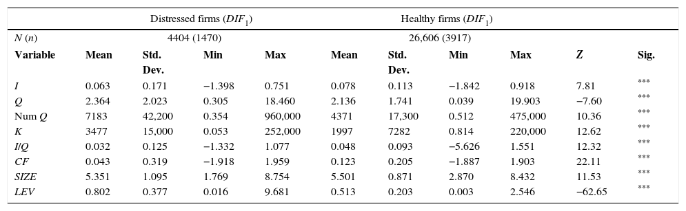
Descriptive statistics II.

	Distressed firms (DIF1)				Healthy firms (DIF1)
N (n)	4404 (1470)				26,606 (3917)
Variable	Mean	Std. Dev.	Min	Max	Mean	Std. Dev.	Min	Max	Z	Sig.
I	0.063	0.171	−1.398	0.751	0.078	0.113	−1.842	0.918	7.81	^***
Q	2.364	2.023	0.305	18.460	2.136	1.741	0.039	19.903	−7.60	^***
Num Q	7183	42,200	0.354	960,000	4371	17,300	0.512	475,000	10.36	^***
K	3477	15,000	0.053	252,000	1997	7282	0.814	220,000	12.62	^***
I/Q	0.032	0.125	−1.332	1.077	0.048	0.093	−5.626	1.551	12.32	^***
CF	0.043	0.319	−1.918	1.959	0.123	0.205	−1.887	1.903	22.11	^***
SIZE	5.351	1.095	1.769	8.754	5.501	0.871	2.870	8.432	11.53	^***
LEV	0.802	0.377	0.016	9.681	0.513	0.203	0.003	2.546	−62.65	^***

	Distressed firms (DIF2)				Healthy firms (DIF2)
N (n)	4868 (1770)				26,142 (3823)
Variable	Mean	Std. Dev.	Min	Max	Mean	Std. Dev.	Min	Max	Z	Sig.
I	0.044	0.160	−1.371	0.836	0.082	0.114	−1.842	0.918	27.33	^***
Q	2.607	2.327	0.039	18.683	2.086	1.652	0.072	19.903	−11.64	^***
Num Q	880	5254	0.354	147,000	5495	24,400	0.904	960,000	50.18	^***
K	477	2699	0.053	80,300	2530	9506	0.814	252,000	56.36	^***
I/Q	0.018	0.147	−5.626	1.451	0.051	0.085	−1.602	1.551	32.70	^***
CF	−0.141	0.356	−1.918	1.959	0.159	0.152	−1.838	1.903	76.14	^***
SIZE	4.822	0.771	1.769	8.065	5.602	0.878	2.870	8.754	55.88	^***
LEV	0.560	0.401	0.003	9.681	0.553	0.219	0.004	3.599	6.81	^***

	Distressed firms (DIF3)				Healthy firms (DIF3)
N (n)	2437 (988)				23,100 (2845)
Variable	Mean	Std. Dev.	Min	Max	Mean	Std. Dev.	Min	Max	Z	Sig.
I	0.040	0.163	−1.398	0.742	0.078	0.112	−1.816	0.832	16.54	^***
Q	2.634	2.443	0.193	18.683	2.066	1.602	0.039	19.875	−8.28	^***
Num Q	900	4802	1.251	134,000	5827	25,600	0.512	960,000	37.09	^***
K	484	2806	0.579	72,400	2673	9774	1.207	252,000	41.63	^***
I/Q	0.016	0.166	−5.626	1.077	0.049	0.086	−1.602	1.551	20.07	^***
CF	−0.046	0.366	−1.796	1.959	0.141	0.168	−1.824	1.894	33.64	^***
SIZE	4.860	0.771	2.782	7.965	5.643	0.864	3.122	8.754	41.15	^***
LEV	0.739	0.469	0.006	9.681	0.539	0.205	0.003	2.392	−26.85	^***

Z is the Wilcoxon rank-sum test.

***

A level of significance of 0.01.

Table 4.

Descriptive statistics III.

	Distressed firms (DIF1) Q > 1				Distressed firms (DIF1) Q < 1						Healthy firms (DIF1) Q > 1				Healthy firms (DIF1) Q < 1
N (n)	3879 (1348)				525 (291)						22,378 (3744)				4228 (1289)
Variable	Mean	Std. Dev.	Min	Max	Mean	Std. Dev.	Min	Max	Z	Sig.	Mean	Std. Dev.	Min	Max	Mean	Std. Dev.	Min	Max	Z	Sig.
I	0.068	0.168	−1.398	0.751	0.021	0.188	−0.992	0.742	−7.67	^***	0.082	0.112	−1.842	0.918	0.055	0.112	−1.438	0.820	−18.64	^***
Q	2.568	2.073	1.000	18.460	0.858	0.126	0.305	0.999	−37.24	^***	2.384	1.791	1.000	19.903	0.819	0.147	0.039	1.000	−103.29	^***
Num Q	7986	44,900	0.354	960,000	1249	3792	1.156	30,900	−10.58	^***	5067	18,700	1.677	475,000	685	2985	0.512	62,900	−48.97	^***
K	3760	15,900	0.053	252,000	1392	4141	1.285	32,300	−2.44	^**	2230	7798	0.814	220,000	767	3177	1.897	65,700	−24.41	^***
I/Q	0.033	0.099	−1.077	0.631	0.021	0.239	−1.332	1.077	−0.32		0.044	0.069	−0.998	0.808	0.067	0.169	−5.626	1.551	19.58	^***
CF	0.043	0.330	−1.918	1.959	0.047	0.221	−1.602	1.105	−5.13	^***	0.136	0.209	−1.887	1.903	0.056	0.167	−1.713	0.728	−45.41	^***
SIZE	5.384	1.116	1.769	8.754	5.105	0.883	3.122	7.471	−4.99	^***	5.568	0.880	2.870	8.432	5.144	0.727	3.261	7.812	−29.73	^***
LEV	0.817	0.391	0.025	9.681	0.687	0.212	0.016	1.477	−8.22	^***	0.517	0.205	0.004	2.546	0.491	0.192	0.003	1.012	−6.70	^***

	Distressed firms (DIF2) Q > 1				Distressed firms (DIF2) Q < 1						Healthy firms (DIF2) Q > 1				Healthy firms (DIF2) Q < 1
N	4049 (1553)				819 (523)						22,208 (3643)				3934 (1200)
Variable	Mean	Std. Dev.	Min	Max	Mean	Std. Dev.	Min	Max	Z	Sig.	Mean	Std. Dev.	Min	Max	Mean	Std. Dev.	Min	Max	Z	Sig.
I	0.051	0.156	−1.371	0.836	0.009	0.175	−1.087	0.812	−10.71	^***	0.086	0.114	−1.842	0.918	0.060	0.108	−1.438	0.820	−6.22	^***
Q	2.976	2.387	1.000	18.683	0.783	0.160	0.039	1.000	−45.20	^***	2.309	1.697	1.000	19.903	0.831	0.140	0.072	1.000	−16.93	^***
Num Q	979	5703	0.354	147,000	393	1748	0.512	14,600	−16.10	^***	6323	26,400	1.677	960,000	821	3296	0.904	62,900	−100.13	^***
K	479	2815	0.053	80,300	467	2034	1.387	17,800	1.61		2816	10,200	0.814	252,000	912	3505	1.285	65,700	−47.60	^***
I/Q	0.021	0.088	−1.077	0.730	0.006	0.300	−5.626	1.451	−0.19		0.047	0.071	−1.049	0.808	0.074	0.138	−1.602	1.551	−25.40	^***
CF	−0.152	0.367	−1.918	1.959	−0.085	0.288	−1.713	1.105	4.30	^***	0.172	0.153	−1.838	1.903	0.084	0.120	−1.710	1.078	20.81	^***
SIZE	4.830	0.783	1.769	8.065	4.781	0.706	3.143	7.185	−1.17		5.671	0.884	2.870	8.754	5.214	0.732	3.122	7.812	−49.92	^***
LEV	0.579	0.424	0.004	9.681	0.468	0.235	0.003	1.477	−6.22	^***	0.558	0.223	0.005	3.599	0.522	0.195	0.004	1.449	−30.95	^***

	Distressed firms (DIF3) Q > 1				Distressed firms (DIF3) Q < 1						Healthy firms (DIF3) Q > 1				Healthy firms (DIF3) Q < 1
N	2062 (862)				375 (249)						19,497 (2730)				3603 (992)
Variable	Mean	Std. Dev.	Min	Max	Mean	Std. Dev.	Min	Max	Z	Sig.	Mean	Std. Dev.	Min	Max	Mean	Std. Dev.	Min	Max	Z	Sig.
I	0.046	0.160	−1.398	0.732	0.007	0.178	−1.087	0.742	−5.59	^***	0.083	0.112	−1.816	0.832	0.055	0.112	−1.438	0.820	−17.53	^***
Q	2.961	2.521	1.000	18.683	0.835	0.144	0.193	0.999	−30.85	^***	2.296	1.642	1.000	19.875	0.820	0.147	0.039	1.000	−95.51	^***
Num Q	960	5103	2.275	134,000	571	2559	1.251	30,900	−8.08	^***	6745	27,700	1.990	960,000	858	3363	0.512	62,900	−47.63	^***
K	457	2814	0.579	72,400	633	2763	2.707	32,300	2.25	^**	2989	10,500	1.207	252,000	960	3598	1.285	65,700	−26.11	^***
I/Q	0.020	0.094	−0.929	0.631	−0.007	0.361	−5.626	1.077	0.81		0.045	0.070	−1.077	0.664	0.068	0.144	−1.602	1.551	17.68	^***
CF	−0.056	0.379	−1.796	1.959	0.007	0.280	−1.694	1.105	1.71	^*	0.154	0.171	−1.824	1.894	0.070	0.135	−1.713	0.728	−45.34	^***
SIZE	4.860	0.775	2.782	7.965	4.860	0.748	3.392	7.471	0.14		5.717	0.868	3.145	8.754	5.241	0.726	3.122	7.812	−31.16	^***
LEV	0.760	0.497	0.019	9.681	0.626	0.237	0.006	1.263	−4.95	^***	0.545	0.207	0.004	2.392	0.507	0.192	0.003	1.012	−9.13	^***

*

A level of significance of 0.1.

**

A level of significance of 0.05.

***

A level of significance of 0.01.

Table 2 provides descriptive statistics for the whole sample. All the differences are statistically significant. All variables present higher values for firms with Q over one, except the dependent variable of our model (I/Q) which is higher for firms with Q under one.

Table 3 provides information for all variables distinguishing healthy and financially distressed firms. The results show that financially distressed firms invest less, have a higher Tobin's q, smaller cash flows, a smaller size and higher leverage than healthy firms. These results follow the same pattern as Bhagat et al. (2005). The greater value of Tobin's q for firms in financial distress could affect the behavior of our dependent variable. In fact, regarding the variable I/Q, the results show that distressed firms present a smaller value, so they seem not to be able to take advantage of all the investment opportunities they have, at least not in the same way that healthy firms do. So, greater values of Tobin's q lead to greater denominator values and a tendency to underinvestment, as we detected in the results presented in Table 2.

Lastly, there is a need for in-depth analysis so, in Table 4, we present the differences for firms with q over and under one, for both healthy and distressed firms. In the case of healthy firms, the results are similar to those previously obtained for the whole sample, presented in Table 2 (higher values for all the variables except I/Q for firms with Q over one). However, for financially distressed firms the behavior of the variable I/Q is not the same, since we do not observe statistically significant differences between firms with Tobin's q over and under one.

These results suggest that healthy and distressed firms have different investment behavior, but we need to test these findings with multivariable analysis in order to take into account all the variables that might affect this behavior.

Results

Table 5 shows the results of the analysis proposed in model 1.

Table 5.

Results of panel data analysis.

	(1)	(2)	(3)
Dependent variable	I/Q	I/Q	I/Q
CF	0.0501	0.1033^*	0.0667^**
	(0.88)	(1.66)	(2.01)
SIZE	−0.0182	−0.0488	−0.0015
	(−0.46)	(−0.89)	(−0.04)
LEV	−0.0473^*	−0.0465	−0.0667^*
	(−1.92)	(−0.76)	(−1.87)
DIF1	−0.2294^**
	(−2.50)
DIF2		−0.1429^**
		(−2.46)
DIF3			−0.1356^**
			(−2.00)
DIF1*QD	0.2181^**
	(2.22)
DIF2*QD		0.1389^**
		(2.40)
DIF3*QD			0.1308^*
			(1.74)
CONSTANT	0.3371	0.3062	0.0991
	(1.48)	(0.65)	(0.49)
β4 + β5	−0.0113	−0.0039	−0.0048
	(−0.66)	(−0.23)	(−0.37)
SECTOR	5.23^***	1.33	0.63
COUNTRY	0.42	0.65	0.63
YEAR	8.29^***	1.64^*	53.62^***
m1	−4.42^***	−3.85^***	−4.54^***
	[0.000]	[0.000]	[0.000]
m2	−0.28	0.17	−0.93
	[0.782]	[0.863]	[0.353]
Hansen	19.57	7.25	36.41
	[0.240]	[0.993]	[0.309]

β₄ + β₅: is the t-statistic for the linear restriction test under the following null hypothesis: H₀: β₄ + β₅ = 0.

SECTOR: Wald's test of the joint significance of the sector's dummy variables. COUNTRY: Wald's test of the joint significance of the country's dummy variables. YEAR: Wald's test of the joint significance of the year's dummy variables. Distributed as a chi-square under the null hypothesis of lack of relationship.

m₁ and m₂ are the 1st and 2nd order serial correlation statistics using residuals in first differences, distributed as N(0,1) under the null hypothesis of non-serial correlation.

Hansen: over-identifying restriction test, distributed as a chi-square under the null hypothesis of no relation between the instruments and the error term.

t-Statistic between brackets and p-values between square brackets.

*

A level of significance of 0.1.

**

A level of significance of 0.05.

***

A level of significance of 0.01.

According to Hypothesis 1a, coefficient β₄ should be negative, reflecting that the firms in distress with fewer investment opportunities reduce the level of investment relative to the investment opportunities. The results show a statistically significant negative relationship between financial distress and the relative investment for firms that have fewer investment opportunities (β₄ is negative and statistically different from zero). In this way, firms in financial distress with fewer investment opportunities present a greater propensity to under-invest. According to Hypothesis 1b, the sum of coefficients (β₄ + β₅) should be positive, reflecting that the firms in distress with greater investment opportunities increase the level of investment relative to the investment opportunities. However, the significance test of the sum of coefficients of the interaction variables (β₄ + β₅) is not statistically different from zero. Thus, companies in financial distress which have more investment opportunities show an investment behavior that is not significantly different from that of healthy companies. This assumes that they do not over-invest, but their investment behavior differs from that of the other companies in financial distress. Specifically, for those companies with greater opportunities, the tendency to under-invest disappears, while this tendency remains for firms with fewer investment opportunities.

These results are partially consistent with the theoretical proposals of White (1996), who defended that firms in financial distress could have problems of over- and under-investment. Some papers have addressed this issue indirectly, finding under-investment problems under different circumstances: when ex-ante bankruptcy costs exists (Pindado et al., 2008) or for financially distressed firms if they operate at a loss (Bhagat et al., 2005). Our results add additional evidence supporting the idea that this investment behavior of financially distressed firms is conditioned by their own investment opportunities. In fact, our findings support under-investment but not over-investment behavior.

Regarding the control variables, the results show a positive and statistically significant relationship for cash flow (CF) in models in columns (2) and (3) of Table 5, so that firms with higher cash flow have a greater propensity to over-invest (Jensen, 1986). Lastly, we find that in models in columns (1) and (3) of Table 5 there is a negative relationship between leverage and the level of investment. This result is similar to that obtained by Lang et al. (1996), who found that there is a negative relation between leverage and future growth of the firms.

These results are in line with the proposition of this study, showing that the investment behavior of firms in distress can be conditioned by their investment opportunities. Thus, firms with fewer opportunities have a propensity to under-invest, showing how managers tend to forego profitable projects if it will not provide a result sufficient to avoiding bankruptcy. However, this situation does not hold in the case of companies with more opportunities, since in this case the investment behavior of firms in distress is no different from that of healthy companies.

Robustness tests

In order to control the robustness of the results, we perform two complementary analyses.

In the first one we test model 1, but dividing the sample according to the value of the Tobin's q instead of using an interaction term. So, we test the model considering firms with Q values over and under one, and with Q values over and under the median value of Q. The model follows this specification:

Model 2:

Using this alternative specification, we prevent our results from being biased due to the introduction of an interaction term of two dichotomous variables (QD and DIF) in the original model (model 1). In this case, we use OLS estimation using the Huber/White/sandwich estimator of the variance–covariance matrix, so the test is robust to an unspecified form of heteroscedasticity. We have to use OLS because we split the sample in two different parts, so we do not have consecutive observations for all firms. If GMM panel data were used, we could only analyze firms with at least five consecutive years with Q over or under one (or under or over the median) in each case. Table 6 provides the results of these analyses.

Table 6.

Robustness test (sample divided according to Tobin's q).

	Model 1 (Q > 1)			Model 1 (Q < 1)			Model 1 (Q > median)			Model 1 (Q < median)
Dependent variable	I/Q			I/Q			I/Q			I/Q
	Coef	Coef	Coef	Coef	Coef	Coef	Coef	Coef	Coef	Coef	Coef	Coef
CF	0.0137^***	0.0020	0.0120^***	0.1542^***	0.1306^**	0.2153^***	0.0087^***	0.0024	0.0060^**	0.1021^***	0.0835^***	0.1400^***
	(5.14)	(0.66)	(3.78)	(2.95)	(2.42)	(3.01)	(3.75)	(0.86)	(2.37)	(4.51)	(3.56)	(4.52)
SIZE	0.0026^***	0.0014^**	0.0014^**	0.0100^**	0.0099^**	0.0104^*	0.0023^***	0.0014^***	0.0011^**	0.0046^***	0.0035^***	0.0036^*
	(4.98)	(2.53)	(2.27)	(2.53)	(2.45)	(1.93)	(4.81)	(2.81)	(2.01)	(3.50)	(2.65)	(1.96)
LEV	0.0024	0.0002	0.0040^*	0.0143	−0.0079	0.0206	−0.0014	−0.0011	0.0004	−0.0013	−0.0101	0.0065
	(1.10)	(0.09)	(1.82)	(0.66)	(−0.39)	(0.67)	(−0.80)	(−0.67)	(0.24)	(−0.15)	(−1.23)	(0.55)
DIF1	−0.0069^***			−0.0411^***			−0.0009			−0.0187^***
	(−3.88)			(−3.63)			(−0.54)			(−4.63)
DIF2		−0.0189^***			−0.0372^***			−0.0101^***			−0.0270^***
		(−10.64)			(−3.66)			(−5.81)			(−5.88)
DIF3			−0.0168^***			−0.0527^***			−0.0113^***			−0.0306^***
			(−7.08)			(−2.71)			(−5.29)			(−3.95)
CONSTANT	0.0352^***	0.0468^***	0.0431^***	−0.0065	0.0087	−0.0077	0.0266^***	0.0340^***	0.0359^***	0.0352^***	0.0486^***	0.0350^***
	(10.97)	(14.08)	(12.14)	(−0.37)	(0.48)	(−0.39)	(8.99)	(10.91)	(11.09)	(5.17)	(7.14)	(4.79)
SECTOR	20.40^***	16.15^***	21.43^***	8.04^***	9.34^***	3.72^**	16.55^***	13.19^***	10.87^***	10.08^***	13.00^***	5.86^***
COUNTRY	33.63^***	29.46^***	22.06^***	5.67^***	6.65^***	4.38^***	24.96^***	23.51^***	15.90^***	6.10^***	5.64^***	3.32^***
YEAR	151.49^***	146.12^***	147.80^***	26.58^***	27.21^***	29.22^***	83.16^***	80.83^***	88.11^***	89.78^***	90.95^***	89.97^***
R^2	0.07	0.08	0.09	0.08	0.09	0.12	0.07	0.07	0.09	0.08	0.08	0.10
F	89.23^***	94.25^***	86.28^***	19.16^***	18.93^***	18.36^***	51.16^***	52.65^***	51.48^***	54.57^***	55.07^***	52.04^***

SECTOR: Wald's test of the joint significance of the sector's dummy variables. COUNTRY: Wald's test of the joint significance of the country's dummy variables. YEAR: Wald's test of the joint.

Significance of the year's dummy variables. Distributed as a chi-square under the null hypothesis of lack of relationship.

t-Statistic between brackets.

*

A level of significance of 0.1.

**

A level of significance of 0.05.

***

A level of significance of 0.01.

The results are in line with those obtained in our previous analysis. Table 6 shows how the influence of the variable DIF varies according to the value of Tobin's q. The value of the coefficient associated with this variable is negative and significant for both firms with Q values over and under one. However, this negative effect is much more intense for firms with Tobin's q under 1 (the coefficients are from 2 to 6 times more intense depending on the model). When we divide firms according to the median, the differences are even bigger (in this case, even the DIF₁ variable is not significant for firms with Q values over the median). According to these results, firms in financial distress with fewer investment opportunities present a greater propensity to under-invest, as we showed in our previous panel data analysis.

The second robustness analysis is performed using the traditional measure of investment over replacement value of assets (I) as dependent variable, dividing the sample in firms with I/Q over and under the median of their industry. This complementary analysis allows us to control that our results are not biased by the way we measure the firm's investment, I/Q, a new measure proposed in this paper. So, we propose the estimation of the following model, using the traditional measure of investment over replacement value of assets (I), and controlling the over and underinvestment situations using two subsamples: one that includes firms with a greater tendency to overinvest, with greater values of I/Q and the other that includes firms with greater a tendency to underinvest, with smaller values of I/Q.

Model 3⁴:

Table 7 provides the results of these analyses.

Table 7.

Robustness test (sample divided according to the over and under investment intensity).

	Model 1 (I/Q > industry)			Model 1 (I/Q < industry)
Dependent variable	I			I
	Coef	Coef	Coef	Coef	Coef	Coef
CF	0.0050	0.0220^***	0.0163^*	0.0619^***	0.0593^***	0.0776^***
	(0.73)	(2.95)	(1.92)	(8.74)	(7.24)	(9.10)
SIZE	0.0038^***	0.0042^***	0.0071^***	0.0044^***	0.0049^***	0.0046^***
	(3.54)	(3.88)	(6.28)	(4.37)	(4.87)	(4.14)
LEV	0.0105^**	0.0300^***	0.0215^***	−0.0162^***	−0.0290^***	−0.0255^***
	(2.14)	(6.40)	(4.60)	(−3.58)	(−6.75)	(−6.38)
DIF1	0.0350^***			−0.0244^***
	(11.27)			(−7.23)
DIF2		0.0317^***			−0.0077^**
		(8.26)			(−2.28)
DIF3			0.0247^***			−0.0109^**
			(5.87)			(−2.46)
CONSTANT	0.1076^***	0.0934^***	0.0858^***	0.0173^***	0.0207^***	0.0197^***
	(17.46)	(15.01)	(13.16)	(3.09)	(3.68)	(3.30)
SECTOR	17.02^***	11.87^***	12.76^***	32.05^***	30.22^***	16.85^***
COUNTRY	82.70^***	81.79^***	85.82^***	3.13^***	3.80^***	5.84^***
YEAR	7.79^***	7.39^***	11.02^***	41.35^***	42.93^***	44.40^***
R^2	0.06	0.05	0.06	0.07	0.07	0.09
F	39.56^***	35.86^***	38.14^***	34.75^***	34.68^***	35.02^***

SECTOR: Wald's test of the joint significance of the sector's dummy variables. COUNTRY: Wald's test of the joint significance of the country's dummy variables. YEAR: Wald's test of the joint significance of the year's dummy variables. Distributed as a chi-square under the null hypothesis of lack of relationship.

t-Statistic between brackets.

*

A level of significance of 0.1.

**

A level of significance of 0.05.

***

A level of significance of 0.01.

Table 7 shows the influence of financial distress over investment (using I as dependent variable) for firms according to their tendency to over or under invest (i.e. distinguishing whether their I/Q values are over or under the median of their industry). The results show that, in the group of firms with smaller investment values over Q, the variable DIF is negative and significant, so financially distressed firms in this group present a greater propensity to under-invest. However, for the group of firms with I/Q over the industry median, the variable DIF is positive and statistically significant, so in this group financially distressed firms present a greater propensity to overinvest.

Conclusions

This paper analyzes the influence of financial distress on the investment behavior of companies. The study analyzes the different behavior of firms in financial distress, taking into account the differences that may occur among companies in financial distress depending on their investment opportunities.

The results show that the investment behavior is not uniform for all companies facing financial distress, and the propensity to under-invest depends on the investment opportunities available to the company. Thus, firms with greater opportunities that believe that the additional investments can help them to overcome their difficulties do not show differences with respect to the investment behavior of healthy firms when it comes to taking advantage of investment opportunities. However, managers of companies with fewer investment opportunities have a greater propensity to under-invest because they only implement projects that they consider may prevent the company from having to file for bankruptcy. This behavior makes them miss profitable opportunities that would help improve the situation of the company in distress.

This helps to explain why the reorganization processes undertaken by many firms in distress are often unable to prevent their demise. In this sense, the results are particularly relevant at the present time, in light of the reforms that have occurred in bankruptcy laws in different countries, and the economic crisis, which has increased the number of insolvencies worldwide.

Moreover, future extension of this work could study the effect that the way firms deal with financial distress has on their investment behavior. On the one hand, it might be relevant if firms follow an informal procedure or file for bankruptcy (Aybar Arias et al., 2006; Gilson, 1997; González and González, 2000). On the other hand, firms filing for bankruptcy are affected by different insolvency procedures, because bankruptcy laws vary across countries (Davydenko and Franks, 2008; López Gutiérrez et al., 2012).