A Model and Solution Method for Solving the Real-world and Complex Problem of Scheduling Visits to Customers

Abstract

Some of the complex logistical problems faced by companies combine the needs for strategic and tactical decisions concerning the interrelated issues of clustering, scheduling, and routing. Various strategies can be used to solve these problems. We present a problem of this type, involving a company whose fundamental objective is the commercialization of its product in the domestic market. The paper focuses on a model of and method for a solution to the problem of scheduling visits to customers, taking into account the relationship with other phases of product marketing. The model is nonlinear, involves binary and continuous variables, and solved heuristically. Computational experiments show that the proposed solution performed very well for both real-life and theoretical instances.

1

Introduction

This work involves part of a complex real-world logistical problem faced by a company operating on public and private investments whose main objective is the commercialization of its product in the domestic market.

The study’s fundamental practical contribution is solving the real-world problem presented, allowing an improved supply chain through one of its two main activities, the logistics, by combining strategic and tactical decisions. The real-world problem is the partitioning of customers into certain groups and planning visits to these customers over a given time horizon (strategic decisions) and the construction of efficient routes by which to visit the customers (tactical decisions). Theoretically, this problem contains the sub-problems of clustering, scheduling, and vehicle routing and the interdependent complexities imposed by certain restrictions not considered by the literature’s classical models.

Solving the problem while addressing clustering and the location of the warehouse and routing is very complex. There exists an extensive literature on solving integrated problems such as location-routing [1] [2], assignment-routing [3], cluster-routing [4] [5], vehicle and crew scheduling [6], routing-scheduling [7] [8], facility location, and modes inventory [9]. The literature also features complex logistical problems divided into phases with minor levels of complexity. For example, the urban transit network design problem (UTNDP) has been divided into two main sub-problems: routing and scheduling [10]. The transportation scheduling problem for mobile devices described in [11] presents a model with nonlinear time intervals, which is transformed into a mixed integer program (MIP) by the same decomposition principle of Dantzig-Wolfe.

The crew scheduling problem is usually divided into three phases [12]. In [13], we see different methods for the selection and allocation of warehouses to customers. A study of different versions of the assignment problem and their solutions can be found in [14]. The proposed model is mixed integer nonlinear non-convex. A study of heuristic methods for solutions to this kind of model can be found in [15].

This paper summarizes the methodology for solving this problem, divided into phases. Its main contribution is the model and solution for the second phase: the problem of scheduling visits to customers. We have designed an experiment to validate the proposed solution method using information drawn from the real-world problem and have adapted relevant instances from the literature.

The structure of the real-world problem is as follows. The company has a set of points of sale for a product that must be visited every month at a frequency determined by its sales volume by one of the nine company trucks travelling from a central depot to which they must return after their journey. Each customer must always be visited by the same truck. Some customers are visited on the same day by the same truck, as happens when at least one customer associated with a headquarters customer is visited.

There are 4 types of visit frequency, each depending on the customer’s sales volume: weekly (the same day each week, for example every Tuesday), biweekly (two visits per week, which must be Monday and Thursday or Tuesday and Friday), bimonthly (2 times a month, in the first and third weeks or the second and fourth weeks, but always on the same day of the week) and monthly. The trucks are available from Monday to Friday. A month is considered to be 4 weeks with 20 days of delivery.

The length of the truck’s stay with customers is not constant and does not depend on delivery frequency or the amount delivered (the sales volume) but on the type of visit. Though the trucks have a limited capacity, the current restriction is the truck’s total available travel time, not its capacity. Thus, the capacity of the trucks is generally higher than the load equal to the maximum number of customers who can be visited in a day.

2

Methodology

The problem was solved using a heuristic involving three key phases in the order listed below:

• a)

  Customer clustering problem based on the use of clustering techniques.

• b)

  Scheduling visits to customers located in the same cluster in a given period, a month in our case.

• c)

  Vehicle routing with time windows and additional restrictions for each set of customers to be visited each day by the same truck.

These three phases were not resolved by ignoring the others phases; the solution method proposed includes constraints defined by the other phases. In Phase 1, restrictions are taken into account to help the later phases of scheduling visits and to try to balance the volume of monthly visits in each cluster, containing the customers with equal visit frequencies and who must be visited together. This involves constructing clusters with constraints mainly of capacity. Similarly, Phase 2 seeks to achieve well-formulated routes. Phase 3 seeks to minimize the total distance among the customers visited every day to its geometric centroid. In this work, Phase 1 and 3 are not considered. First, a short review of Phase 1 is presented (detailed in [16]) due to the relationship between the instance structures used in the design of experiments developed to solve the problem of scheduling visits to customers and the clusters obtained in the first phase.

2.1

Phase 1: Building the customer cluster

To solve the problem of the formation of distribution areas with capacity constraints, we decided to follow a philosophy similar to that proposed by Pacheco and Beltran [17] and Éric Taillard in [18]. They have adapted a k-means method using centroids to provide a clear physical interpretation of a real-world problem (the grouping of geographical areas) and provided the geometric center of each cluster.

The algorithm has two steps:

• a)

  Selecting a number of k initial points (seeds) sufficiently far apart to be considered the initial centroids of the k clusters to be built.

• b)

  Allocating the remaining points (customers) to a cluster or zone one by one according to the philosophy of the k-means algorithm and taking into account the capacity constraints. The capacity of a cluster is the maximum amount of visits that can be performed monthly. The customers who must be visited together are replaced by a new artificial customer with a capacity equal to the sum of all and located on the centroid of all these points.

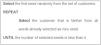
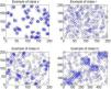
To obtain several solution methods, the two steps described above were designed independently, allowing the possibility of combination. For each step, two different methods were implemented, producing four methods for the creation of clusters or distribution zones. The pseudocode of the algorithms used is described in Figures 1-3. An experiment was designed to validate the performance of the algorithm with regard to the quality of the solutions found and the computational time. The parameters evaluated by the experiment were the number of clusters to be made, the number of customers, and the geographical distribution of the customers divided into three classes using the same notation used by Homberger in [19]:

• a)

  The class of instances where their points are distributed uniformly. This class is denoted by the letter r.

• b)

  The class of instances where their points are concentrated in certain areas of the region where they are located. This class is denoted by the letter.

• c)

  The class of instances where there is a combination of the features of the previous two classes. This class is denoted by the letter rc.

Figure 1.

Pseudocode of Phase 1, Method 1.

Figure 2.

Pseudocode of Phase 1, Method 2.

Figure 3.

Pseudocode of Phase 2, Method 1 and 2.

Figure 4 shows examples of customer distributions. The results show that a variant of the algorithm does not compete with others in terms of solution quality. Moreover, no algorithm is dominated by the others, taking into account all the factors that may influence the performance of the algorithms. However, according to the particular characteristics that present the instances and clusters used to build this problem. The description of the proposed algorithms and the design of experiments is in [16].

Figure 4.

Graphical representation of customers corresponding to instances of class c, r, and rc.

2.2

Phase 2: The scheduling of visits to customers in a given cluster

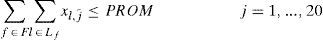
Mathematical model proposed for the assignment of monthly visits to customers.

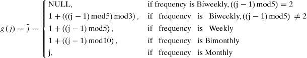
Indices

• j: day of the month

• l: customer

• k: headquarter

• f: frequency

Sets

F: Set of frequencies f, F = {(BS) Biweekly, (S) Weekly, (Q) Bimonthly, (M) Monthly}

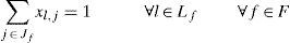
L_f: Set of customers / with frequency f

K: Set of headquarters k

A_k: Set of customers / associated with the headquarter k

J_f: Set day of the month corresponding to the frequency f

Parameters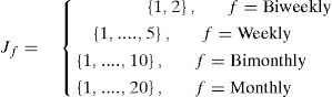

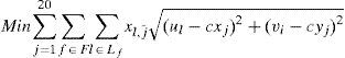
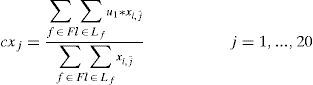
u_i: x coordinate for the customer /

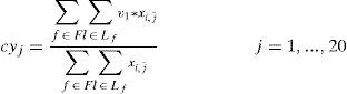
v_j: y coordinate for the customer

Functions

Variables

cx_j : x coordinate for the centroid associated with the day j = 1,...,20

cy_j : y coordinate for the centroid associated with the day j = 1,...,20

Objective function

Constraints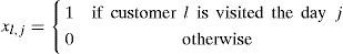

The role of the function g(j) is to link the variables x_l,j for different days j of the month and different frequencies of distribution to reduce the number of variables by not defining 20 variables (days of the month to be considered) for each frequency.

For frequency BS, only two variables are used, for frequency S, five variables, and for frequencies M and Q, ten and 20 are used, respectively.

The objective function minimizes the sum of the distances from the points to be visited every day to its centroid (cx_j, cy_j). This objective function take into account the next phase of building the best daily delivery routes.

In type (1) constraints, every customer should be scheduled in the month according to the frequency of their visits. This does not mean that they are visited only once.

For example, a customer with frequency f = BS has two scheduling possibilities, J_BS = {1, 2}. If the value is 1, visits will occur every week on Mondays and Wednesdays; if it is 2, visits will happen every week on Tuesdays and Fridays, thus eight visits a month. A customer with frequency f = S has five options for scheduling the visits, J_S = {1, 2, 3, 4, 5}.

If the value is 1, visits will occur every week on Mondays; if it is 2, visits will happen every week on Tuesdays; if it is 3, visits will take place every week on Wednesdays.

In type (2) constraints, all customers associated with the same headquarters with equal visit frequencies are visited on the same days of the month.

Type (3) constraints impose a balance in the daily number of visits, according to the total number of visits scheduled in the month.

Type (4) and (5) constraints produce the assignment of the centroids, corresponding to the coordinates x and y, respectively, for each day of the month according to the scheduled visits on those days.

Type (6) and (7) restrictions define the domain of the variables.

2.3

Proposed solution method

The model is highly nonlinear, with binary variables and continuous type. According to the real-word data, one cluster would have 40 continuous variables and approximately 2700 binary variables.

The scope of the real-world problem will likely broaden in the coming years, the company forecasts a substantial increase in the number of customers. We therefore propose a heuristic solution method that uses in one of its steps a well-known exact solution of the integer linear problem as a black box.

The first step is placing the centroids at the coordinate (0, 0) of all customers to be visited each day of the month. With fixed centroids, the model becomes an integer linear programming (ILP) problem solved using software, such as CPLEX.

The values of the variable x_l,j are replaced with the solution obtained in equations (4) and (5) of the centroids. The objective function is updated with the values of the new centroid, and we update the new solution if it is the best so far.

When the algorithm recognizes that it will reach a local optimum, we run an escape routine to diversify the search with random centroids and start another intensification search from these new random centroids.

The escape routine should change the centroid to a far point because it will fall back into the same local optimum (i.e., the same solution) if it is similar.

Figure 5 presents the proposed method in pseudocode.

Figure 5.

Proposed heuristic algorithm in pseudocode.

3

Design of experiment to evaluate the proposed solution method

3.1

Structures of the real-world instances

The values used in the parameters (such as size of the instances, the instances’ structure, and number of clusters to obtain) take into account not only the characterization of the company’s current problem (the clustering and scheduling of customers in a particular city) but also the fact that the same problem will soon occur in others cities, where these parameters may change significantly. For example, in the real problem, the total number of customers is around 9500.

Havana city presently has the most customers with 10 distribution zones, an average of 360 customers per distribution zones, and a maximum of about 650 customers in the most populous zone.

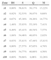
The frequency distribution for deliveries corresponds to the current customers in Havana (Table 1). Although the focus of this paper is the solution to the Havana city problem, we addressed different situations in other provinces where the company is established, as well an expected increase of customers in the coming years.

Table 1.

Frequency distribution for the deliveries.

Zone	BS	S	Q	M
z1	0,00%	56,61%	30,17%	13,22%
z2	0,92%	52,53%	36,87%	9,68%
z3	0,67%	45,30%	39,26%	14,77%
z4	1,48%	35,93%	55,19%	7,41%
z5	6,49%	45,41%	40,54%	7,57%
z6	1,88%	54,46%	40,85%	2,82%
z7	0,93%	35,81%	47,44%	15,81%
z8	0,00%	27,57%	67,65%	4,78%
z9	0,00%	54,77%	40,66%	4,56%
z10	0,00%	59,68%	8,06%	32,26%

The algorithms were tested on a set of instances taken from the literature [16] that involve problems similar to the one facing the company and on instances generated through the characteristics presented in the real-world problem being addressed.

The properties of the instances considered to seek a correlation with the performance of the algorithms are the following:

• a)

  The size of the instances, defined by the number of data (customers) to schedule.

• b)

  The structure of the instances, defined as the characteristics of the geographical distribution of customers in a zone where partitions are to be built.

The structure of the instances comprised the three classes of instances featured in the first section of building clusters.

These instances had between 100 and 1000 customers. Specifically, they had 100, 200, 300, 400, 600, 800, and 1000 customers based on the proposed instances in the literature [16] and considering the previously described classes r, c, and rc.

The frequency of distribution relative to the total number of customers in each instance (BS, S, Q, and M) is measured according to the ten regions where the company has customers at present in Havana city as shown in Table 1.

Thus, we distribute the customers with the same frequencies (biweekly, weekly, biweekly, and monthly) in the ten areas as in the real-world problem.

We test various termination conditions for our heuristic solutions:

• a)

  Stop at the first local optimum (iter1).

• b)

  Stop at the second local optimum (iter2).

• c)

  Stop after finding one local optimum without improving the global optimum (nome1).

• d)

  Stop after finding five consecutive local optimums without improving the global optimum (nome5).

• e)

  Stop after finding 100 local optimums (iter100). With this terminate condition, the heuristic explores a large number of possible local optimums, using a long computation time. This condition term is used as the best-known solution for comparing the quality of the other criteria.

The implementation was developed on a computer with an Intel Pentium 4 3.40GHz using a Linux Ubuntu 11.10 operating system. To solve the exact ILP models was used IBM ILOG CPLEX 12.4 solver.

3.2

Experimental results

Extensive computational tests were conducted to evaluate the performance of the heuristic proposed in terms of the quality of the solution (%gap) compared against the best known solution and the computation time required to reach it.

The number of instances generated and tested was 350. The instances were generated from five sets of coordinates for customers with different distributions, or classes, as presented by [18], using 100, 200, 300, 400, 600, 800, and 1000 customers for each of these classes. Finally, each customer was assigned a frequency of visit according to the probabilities of each of the ten zones of distribution as shown in Table 1.

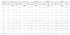
Tables 2, 3, and 4 show the five term conditions evaluated, displaying for each the difference between the solution obtained and the best solution found (%gap), the computing time used in seconds (CPU Time), and the number of local optimums visited (Iter.).

Table 2.

Summary of results by the number of customers.

Instance Type	iter1			iter2			nome1			nome5			iter100
	%GAP	CPU Time	Iter.	%GAP	CPU Time	Iter.	%GAP	CPU Time	Iter.	%GAP	CPU Time	Iter.	%GAP	CPU Time	Iter.
c1	4,92%	9,82	1,00	2,25%	21,69	2,00	1,56%	34,03	2,86	0,53%	122,88	9,17	0,00%	1.505,73	100,00
c2	5,05%	10,74	1,00	2,32%	22,53	2,00	2,05%	36,36	2,69	0,50%	135,69	10,41	0,00%	1.608,46	100,00
r1	2,29%	10,88	1,00	1,55%	23,07	2,00	1,36%	36,69	2,41	0,49%	154,47	9,89	0,00%	1.691,89	100,00
r2	3,33%	10,02	1,00	1,86%	23,67	2,00	1,68%	39,61	2,73	0,57%	142,49	9,30	0,00%	1.552,44	100,00
rc1	4,21%	10,78	1,00	2,30%	22,64	2,00	1,74%	38,27	2,69	0,50%	124,15	9,59	0,00%	1.507,41	100,00
Average	3,96%	10,45	1,00	2,06%	22,72	2,00	1,68%	36,99	2,67	0,52%	135,93	9,67	0,00%	1.573,19	100,00

Table 3.

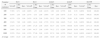
Summary of results by instance type.

Zone Type	iter1			iter2			nome1			nome5			iter100
	%GAP	CPU Time	Iter.	%GAP	CPU Time	Iter.	%GAP	CPU Time	Iter.	%GAP	CPU Time	Iter.	%GAP	CPU Time	Iter.
z1	1,28%	8,54	1,00	0,68%	20,18	2,00	0,50%	37,46	2,71	0,20%	104,17	8,89	0,00%	1.270,79	100,00
z2	3,67%	10,86	1,00	1,82%	23,35	2,00	1,52%	34,76	2,74	0,53%	111,46	8,49	0,00%	1.482,21	100,00
z3	4,59%	9,75	1,00	1,92%	20,06	2,00	1,78%	32,05	2,54	0,58%	123,18	9,97	0,00%	1.301,38	100,00
z4	5,40%	9,10	1,00	2,79%	21,73	2,00	1,89%	39,52	2,83	0,81%	173,40	9,97	0,00%	1.693,38	100,00
z5	6,03%	11,49	1,00	3,83%	24,40	2,00	3,15%	35,97	2,54	0,88%	150,74	9,71	0,00%	1.796,03	100,00
z6	3,78%	7,84	1,00	2,63%	18,72	2,00	2,37%	30,96	2,66	0,58%	119,58	9,23	0,00%	1.440,43	100,00
z7	3,97%	10,19	1,00	2,57%	21,83	2,00	2,53%	38,34	2,51	0,88%	135,02	10,11	0,00%	1.570,63	100,00
z8	5,46%	17,57	1,00	2,30%	36,46	2,00	1,48%	56,90	2,89	0,40%	212,99	10,46	0,00%	2.490,33	100,00
z9	3,10%	10,93	1,00	1,01%	23,31	2,00	0,81%	33,94	2,51	0,18%	125,11	9,77	0,00%	1.494,01	100,00
z10	2,32%	8,20	1,00	1,01%	17,16	2,00	0,74%	30,01	2,80	0,17%	103,68	10,11	0,00%	1.192,67	100,00
Average	3,96%	10,45	1,00	2,06%	22,72	2,00	1,68%	36,99	2,67	0,52%	135,93	9,67	0,00%	1.573,19	100,00

Table 4.

Summary of results by zone type.

Number of customer	iter1			iter2			nome1			nome5			iter100
	%GAP	CPU Time	Iter.	%GAP	CPU Time	Iter.	%GAP	CPU Time	Iter.	%GAP	CPU Time	Iter.	%GAP	CPU Time	Iter.
100	7,76%	0,71	1,00	2,89%	1,53	2,00	2,01%	3,09	2,92	0,75%	8,88	9,70	0,00%	96,98	100,00
200	4,45%	2,04	1,00	2,47%	4,34	2,00	1,96%	7,97	2,60	0,67%	23,45	8,72	0,00%	306,92	100,00
300	4,23%	5,20	1,00	2,45%	10,28	2,00	2,16%	16,12	2,60	0,70%	50,98	9,26	0,00%	643,02	100,00
400	3,54%	7,00	1,00	1,90%	14,18	2,00	1,73%	23,54	2,66	0,64%	73,43	9,26	0,00%	966,40	100,00
600	2,52%	12,47	1,00	1,96%	27,28	2,00	1,62%	40,37	2,62	0,35%	166,88	10,30	0,00%	1.871,33	100,00
800	3,00%	20,11	1,00	1,39%	44,37	2,00	1,16%	74,12	2,72	0,20%	269,49	10,30	0,00%	3.081,42	100,00
1000	2,22%	25,61	1,00	1,32%	57,06	2,00	1,10%	93,74	2,60	0,32%	358,43	10,16	0,00%	4.046,23	100,00
Average	3,96%	10,45	1,00	2,06%	22,72	2,00	1,68%	36,99	2,67	0,52%	135,93	9,67	0,00%	1.573,19	100,00

As Table 2 shows, grouping the solutions according to the number of customers reveals that, as the number of iterations increases, the computation time required increases as well. Likewise, the quality of the solution improves as the number of iterations increases as is reflected by the decreasing %gap.

The increase in computation time due to the number of customers occurred because the ILP model that is solved in each iteration increases the number of binary variables as the number of customers’ increases.

In Table 3, we see significant differences in the quality of the solution when customers are distributed according to the classes r, c, and rc.

Table 4 shows that different zones, each one with a different frequency, had different solution qualities through our heuristic algorithm.

Tables 2, 3, and 4 show that the conditions of terminate nome5 and iter100 show no differences in solution quality but that the computational time is an order of magnitude lower with nome5.

To find a balance between computation time and solution quality, it is recommended to use the term nome5 condition. A lower bound for the non-convex mixed integer nonlinear model was not reported, because it is difficult to obtain a good lower bound using the current state of the art software for these cases. Experiment with smallest cases less than 100 customers showed that our algorithm found nearly optimal solutions.

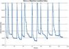
Figure 6 shows how the objective function evolves with respect to the number of iterations. Each iteration showed an improvement in the value of the objective function, ending on a point where it was trapped into a local optimum. When this happens, the diversification routine should be run by the heuristic in order to escape and explore other solutions within the feasible region. This procedure ends according to the terminate condition used.

Figure 6.

Objective function value by the number of iterations.

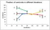
Figure 7 shows an example involving customers who need to be visited once a week. The evolution of the algorithm is seen in each one of the five paths corresponding to the centroids of the five days of the week. Initially, all centroids are clustered in one point at the center and then move toward forming clusters of customers.

Figure 7.

The position of the centroids in different iterations of the algorithm.

In the last iteration, the centroids are located exactly at the center of the cluster, corresponding to the optimal solution for this example.

4

Conclusions and future work

This study proposes to solve a real-world problem using highly complex logistics not yet attempted in the literature.

The results of customer clustering and scheduling of monthly visits have meet the requirements of the company, particularly that of sales management.

The experiment was designed using the types of instances that the company has identified as current as well as others that will need to be addressed in the near future.

Future work is needed to address the routing phase and integrate it into a decision support system using information from a geographic information system.

Acknowledgements

This work was partially supported by the Pontificia Universidad Javeriana Cali and the Universidad del Bío-Bío. This support is gratefully acknowledged. We also thank the anonymous reviewers for their helpful comments.