


The aim of this article attempts to propose an advanced design of driver assistance system which can provide the driver advisable information about the adjacent lanes and approaching lateral vehicles. The experimental vehicle has a camera mounted at the left side rear view mirror which captures the images of adjacent lane. The detection of lane lines is implemented with methods based on image processing techniques. The candidates for lateral vehicle are explored with lane-based transformation, and each one is verified with the characteristics of its length, width, time duration, and height. Finally, the distances of lateral vehicles are estimated with the well-trained recurrent functional neuro-fuzzy network. The system is tested with nine video sequences captured when the vehicle is driving on Taiwan’s highway, and the experimental results show it works well for different road conditions and for multiple vehicles.
Traffic problems are becoming more and more serious in most countries. To reduce traffic accidents and improve the vehicle ride comfort, many papers have been published in recent years [1][2].
Side impact collision is one of the common types of car accident. This mostly happens when vehicles change their lanes, or merge into the highway. These accidents take place when the approaching vehicle drives into the blind spot of the rear view mirrors or the driver gets distracted. Lateral vehicle detection and distance measurement will help the driver to increase the driving safety.
There have been many related studies in the research of front lane line detection [3-8]. Hough transform and improved algorithms are usually used to find the best fitting lines of land markers [6-8]. In lane line detection of adjacent lane, Sobel masks are used to get the edge pixels, and compute the location of representative edge pixels of lane marking at each scan line [9]. Then, the least-square method [9] and the RANSAC method [10] are used to estimate the linear equation of the lane line from these edge pixels. Lateral vehicle detection is used for providing the vehicle information on the adjacent lane. Mei transforms the region of interest on the lane to a rectangular area with lane-based transformation [11]. Each detected object in this area is verified with its features, such as length, width, and height. Díaz et al. exploit the difference of optic-flow pattern between the static object and overtaking vehicle to get the motion-saliency map and compute the vehicle’s position [12]. Lin et al. use the part-based features to evaluate the existence probability of vehicles [13]. For estimation of the vehicle distance, many researches convert the camera coordinate of acquired image to world coordinate [14-15]. Lai and Tsai use the shape information of rear wheel to estimate the distance. After Hough transformation, the shape of wheel is an ellipse, and the center of the ellipse is used to determine the relative position of the lateral vehicle [15].
In this paper we set up a camera at the left side rear view mirror of the vehicle to monitor road conditions, and design a driver assistance system which is based on image processing techniques.
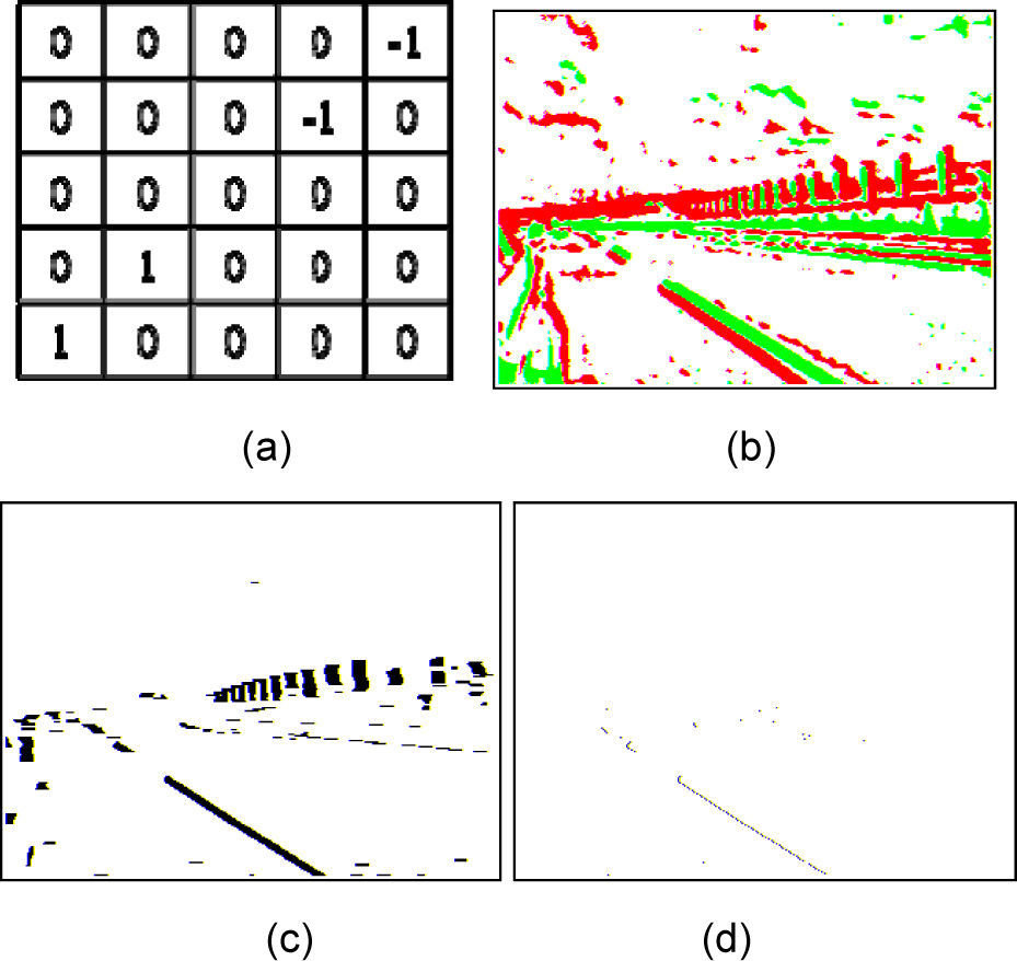
2Adjacent lane-line detectionThe lane-line detection is intended to extract the lane markers without previously knowing the internal or external parameters of the mounted camera. When the vehicle navigates in the middle of the lane, the lane boundary on the left side shown in the captured image will tilt to the left in vertical direction. Based on this feature, we define a 5x5 tilt mask illustrated in Figure 1(a), and apply it on the gray-level image to retrieve the edge pixels in the tilt direction. If the calculated value is greater than thp, the color of the edge pixel will be set to green (positive edge). While the value is less than thn, the color will be set to red (negative edge). The derived image is displayed in Figure 1(b), and the thresholds for positive and negative edges are set to 10 and -10 in the following experiments. Moreover, if the distance between positive and negative edges, marked with green and red colors, is less than ten, the pixels between them will be colored black. Then, all pixels except black ones in this image are colored white to get the binary image, which is shown in Figure 1(c). A region near the host vehicle is pre-specified. Within this region, a fan scanning detection method is applied to exclude noise data. This method scans the edge pixels from the bottom to top, and left to right. The first encountered pixel in each row is saved, but all the other pixels at the same row are deleted. The derived edge points are shown in Figure 1(d).
 The tilt mask. (b) The image of green and red edges. (c) The image of black edges. (d) The image of the reduced edge pixels.")
The points in Figure 1(d) are scanned from bottom to top, and the continuous and adjacent edge points of same direction are grouped into line segments. This is done by checking the bottom-right and limit-sized area of each encountered edge pixel. If there exists an endpoint of line segment created previously, the encountered pixel will accede to the found line segment. Otherwise, the encountered pixel will create a new line segment. The followings are the detail descriptions of the method.
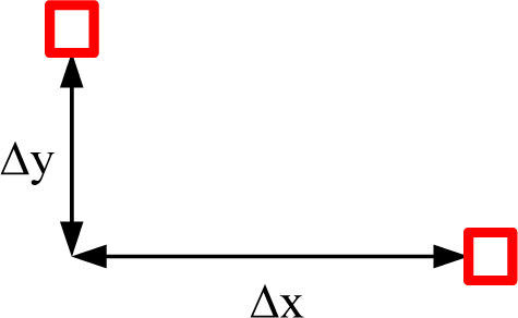
Step 1: Calculate the distances Δx and Δy, as depicted in Figure 2, in coordinates between the current edge pixel and the previous edge pixel. If 0 ≦ Δx<thx and 0 ≦Δy<thy, the point accedes to the line segment of the previous edge pixel, where the thx and thy are predefined thresholds. Otherwise, step 2 is used.

Step 2: Calculate the distances between the current edge pixel and end points of the created line segments. If 0 ≦ Δy ≦ thy and 0 ≦ Δx ≦ thx, the current point accedes to the nearest line segment. If not, this edge pixel is used to create a new line segment.
Step 3: Based on the result of the two prior steps, the situation Δx=0 is not permitted to sequentially appear twice or more to avoid finding out a vertical line segment.
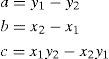
Next, we sort the line segments by their lengths in descending order. The longest segment’s start point (x1, y1) and end point (x2, y2) are taken to estimate a straight line with Eq. (1), where a, b, c are three factors in the straight line equation ax+by+c=0.
Then, we combine other line segments with the longest measurement. From the second longest to the shortest segment, a validation will be proceed to determine whether to merge with the longest line segment. The steps for the merger are as follow:
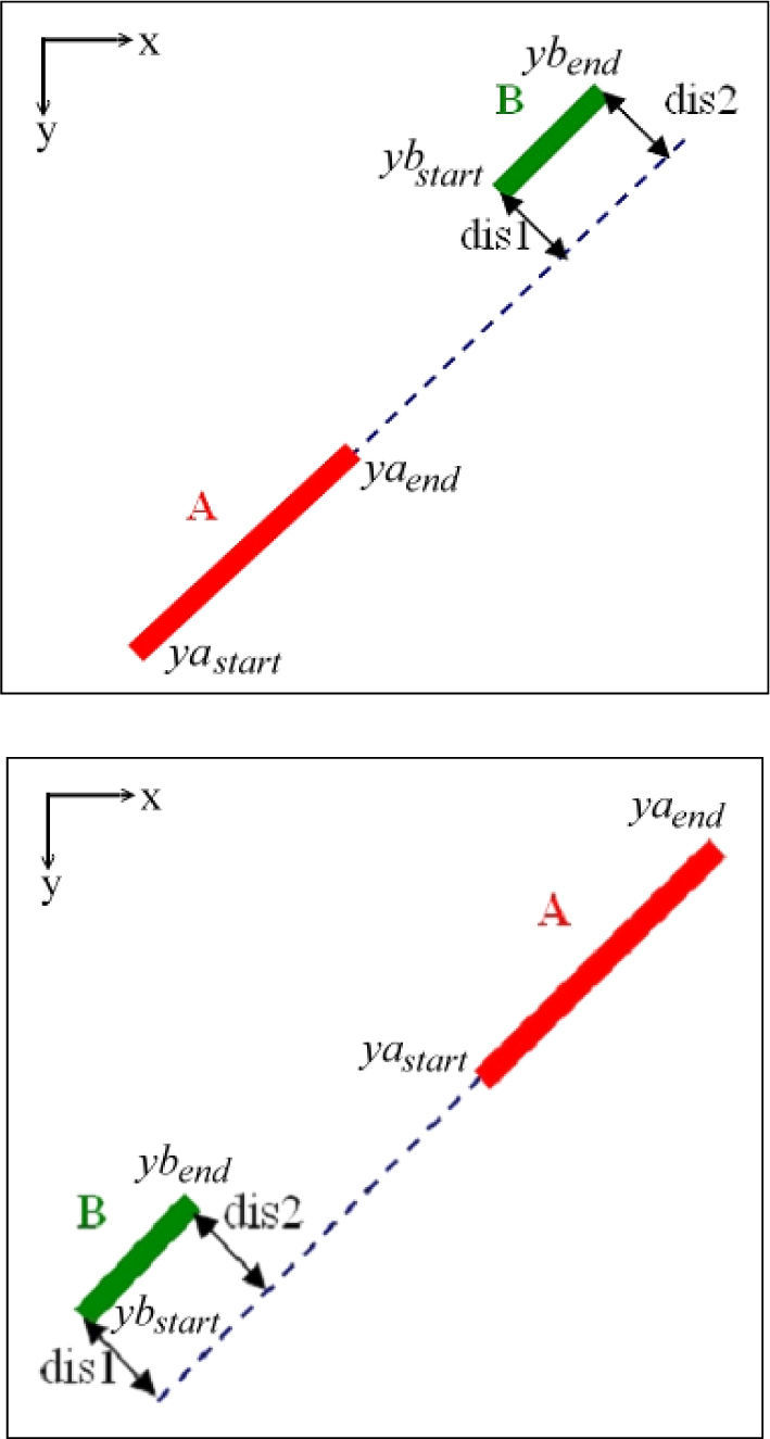
Step 1: The longest line segment will be retrieved first to get the coordinates of the start point and end point (the line segment A in Figure 3).

Step 2: These two points are used to estimate a straight line (the dotted line). Its factor calculation formula is shown in Eq. (1).
Step 3: Then the coordinates of the start point and end point are taken from the checked segment (the B line segment).
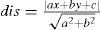
Step 4: The distances, dis1 and dis2, from these two points to the estimated straight line in Step 2 are calculated as follows:
Step 5: If dis1<th1, dis2<th2, the two line segments will combine together to form a new segment.
As the road is not straight, the two line segments may not be aligned in a straight line (the A, B line segment). Therefore, the thresholds th1 and th2 will be adjusted, both of which depend on the distance between the two line segments. That is, the further the distance, the greater the thresholds and it is defined as follows:

In Eq. (3), yastart and yaend are the y-coordinates of the start point and the end point of the longest line segment, respectively, whereas ybstart and ybend represent the checked line segment. After the combining process, the slope of the longest segment is calculated using Eq. (4), where (x1, y1) represents the start point and (x2, y2) represents the end point of the longest segment.

Finally, we use the start point, the end point, and the slope to draw the lane line.
3Distance measurement of lateral vehicleThe detection method for neighboring vehicle is based on the Mei’s method [11], but we add and modify some steps to enhance the detection performance. In this method, the region of interest (ROI) on the lane is transformed into a rectangular area by lane-based transformation [16-17]. Each connected component in this area will be verified with its features, such as length, width, time duration, and height, to determine whether it is a vehicle.
3.1Vehicle detectionFor vehicle detection, the cumulative histogram of gradient magnitude in the road surface area is calculated, and the gradient magnitude at point (x, y) is defined by Eq. (5).

In digital image processing, these magnitudes can be calculated by 3x3 Sobel’s masks. We take magnitude i, where it has accumulated over 80% amount of total points, as the threshold in our experiment. If the gradient magnitude of the pixel is greater than threshold i, the color of the pixel will be set to white. Otherwise, the color will be black.
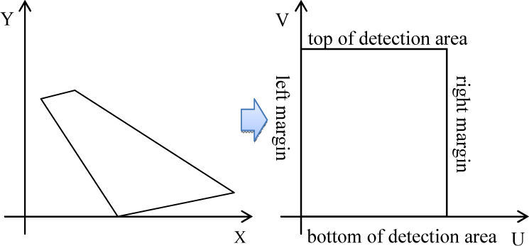
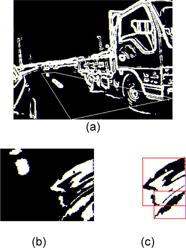
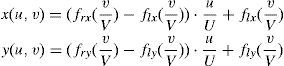
As indicated in Figure 4, a backward rectangle area from the same position at the rear of host vehicle is taken as the ROI. The length of the rectangle is 30meters, and the width is equal to the width of the lane. Then, the ROI is transformed into a rectangular area with lane-based transformation, where the transformed area looks like a vertical view of original region. The concept of lane-based transformation is depicted in Figure 4. The captured image in X-Y plane is converted into the image in the defined U-V plane, and the left and right margin lines of ROI are represented by equations: fl(t)=[flx(t), fly(t)]T and fr(t)=[frx(t), fry(t)]T, where t∈[0,1]. Then, the upper and lower margin lines are represented by equations: fupper(t’)=(fr(1)-fl(1))t’+fl(1) and flower(t’)=(fr(0)-fl(0))t’+fl(0), where t’∈[0,1], t=v/V and t’=u/U. With Eq. (6), each pixel in U-V plane is mapped from pixel in X-Y plane. The binarization image is shown in Figure 5(a) and the transformed image of ROI is shown in Figure 5(b).

 Binarization image. (b) Lane-based transformed image. (c) Bounding boxes.")
Next, the 8-adjacent connectivity is used for image segmentation. In this step, connected components in the transformed image are retrieved, and labeled with different values. As demonstrated in Figure 5(b), a vehicle may be divided into multiple connected components after binarization, and be identified as multiple vehicles by the system. Thus, we re-combine these components, which may belong to the same vehicle, to form a bigger component with the following rule. For each component in U-V plane, we find its bounding box, shown in Figure 5(c). If the bounding boxes overlap, their included components will be combined as a new one.
3.2Vehicle verificationWhen the vehicle travels on the leftmost lane, the solid line painted on the ground may be misjudged as a car when it appears in the detection area. Therefore, we have added the length and the time duration inspections to the vehicle verification in addition to Mei‘s method of width and the height examination. These new inspections can be used to determine whether the vehicle is on the leftmost lane.
In this step, the connected components are examined on its length, width, height, and duration. An unreasonable value of the feature means that the component should not be a candidate of vehicle and would be filtered out. In width examination, we use the width of transformed ROI as a base width, and multiply it with ratios to get the lower bound and upper bound of vehicle width. In the following experiment, the ratios are set to 0.2 and 0.8.
Then, when driving on the leftmost lane, the roadside railings and solid line painted on the road may get into the ROI and be detected as a candidate of vehicle incorrectly. Since the railings and solid line would be transformed as a connected component with a very long length, we can filter out these objects.
Afterwards, the object, whose corresponding connected component passes the width and length inspections, will be inspected in the image of X-Y plane. Using the edge continuity of the object, its sum HL of height and length can be derived. Moreover, the length L of the object is obtained from the length of corresponding bounding box in U-V plane. Hence, the height H of the object is determined by subtracting L from HL. If the object has a feature of height, the found component in UV plane is not a shadow or other noise on lane.
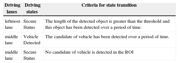
Finally, non-vehicle objects, such as shadows and pavement markings, will enter the ROI for a short period of time. On the other hand, a long solid line will be detected in the ROI within a continuous period of time when the vehicle is traveling in the leftmost lane. Objects of different type have different time durations in the ROI. For this reason, we define different driving states and driving lanes. All the driving lanes and states are tabulated in Table 1. If a new state is detected, the state of the vehicle alters to the new state after it has been detected over a period of time.
Driving lanes, driving state, and criteria for state transition.
| Driving lanes | Driving states | Criteria for state transition |
|---|---|---|
| leftmost lane | Secure Status | The length of the detected object is greater than the threshold and this object has been detected over a period of time. |
| middle lane | Vehicle Detected | The candidate of vehicle has been detected over a period of time. |
| middle lane | Secure Status | No candidate of vehicle is detected in the ROI |
With these methods mentioned above, the non-vehicle objects can be easily filtered out.
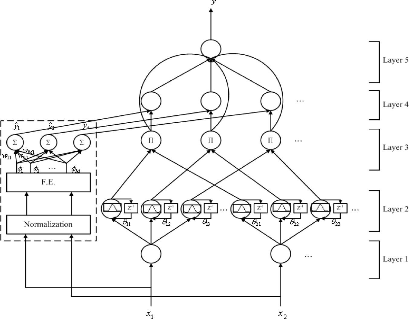
3.3Distance measurement using RFNFNFor distance measurement, we take field measurements to observe the relationship between the pixel distance in image and the real distance, which is non-linear curve. Therefore, we use the measurement data as a training data set for the recurrent functional neuro-fuzzy network (RFNFN)[18], where the structure of the RFNFN model is illustrated in Figure 6. By using the well trained RFNFN, we can calculate the real distance of the detected vehicle from the pixel distance in the image.

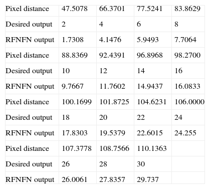
In X-Y plane, the bottom of U-V plane is located at the line which extends from the rear line of the host vehicle. When target vehicle detected in U-V plane, we transform the bottom lines of the target and of the U-V plane reversely to get two lines in X-Y plane. Then, the pixel distance is the distance between these two lines. We start measuring the pixel distance of the target vehicle which is 2meters away from the rear of the host vehicle, and repeat this measurement every two meters backward until the target vehicle is 30meters away. The measurement results of pixel distances (in pixel) and real distance (in meter) are tabulated in Table 2.
The training and output data of RFNFN.
| Pixel distance | 47.5078 | 66.3701 | 77.5241 | 83.8629 |
| Desired output | 2 | 4 | 6 | 8 |
| RFNFN output | 1.7308 | 4.1476 | 5.9493 | 7.7064 |
| Pixel distance | 88.8369 | 92.4391 | 96.8968 | 98.2700 |
| Desired output | 10 | 12 | 14 | 16 |
| RFNFN output | 9.7667 | 11.7602 | 14.9437 | 16.0833 |
| Pixel distance | 100.1699 | 101.8725 | 104.6231 | 106.0000 |
| Desired output | 18 | 20 | 22 | 24 |
| RFNFN output | 17.8303 | 19.5379 | 22.6015 | 24.255 |
| Pixel distance | 107.3778 | 108.7566 | 110.1363 | |
| Desired output | 26 | 28 | 30 | |
| RFNFN output | 26.0061 | 27.8357 | 29.737 |
The training process continues for 500 iterations. Only 4 rules are generated in the RFNFN model after learning. The RMS error of the output data of RFNFN is 0.398905. The obtained fuzzy rules are as follows:
Rule - 1 : IF x1 is μ(78.0311, 31.6539) THEN ŷ1 = 15.6751 x1+0.142648 sin(π x1)−8.30689 cos(π x1) Rule - 2 : IF x1 is μ(145.135, 34.4117) THEN ŷ2=23.7701 x1+0.471216 sin(π x1) −24.6887 cos(π x1) Rule - 3 : IF x1 is μ(45.1327, 15.8387) THEN ŷ3=1.83058 x1+3.13031 sin(π x1)+4.24375 cos(π x1) Rule - 4 : IF x1 is μ(83.1262, 18.263) THEN ŷ4=1.85151 x1+4.94633 sin(π x1)+4.69246 cos(π x1)
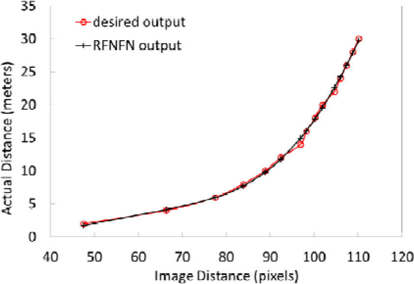
As plotted in Figure 7, the desired output and the FNFN output are almost fully equivalent. The estimated real distance is also tabulated in Table 2. From the results, the proposed RFNFN can be used as a feasible and effective system for distance detection.
4Experimental results
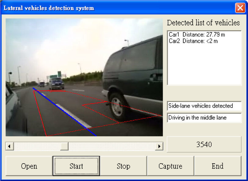
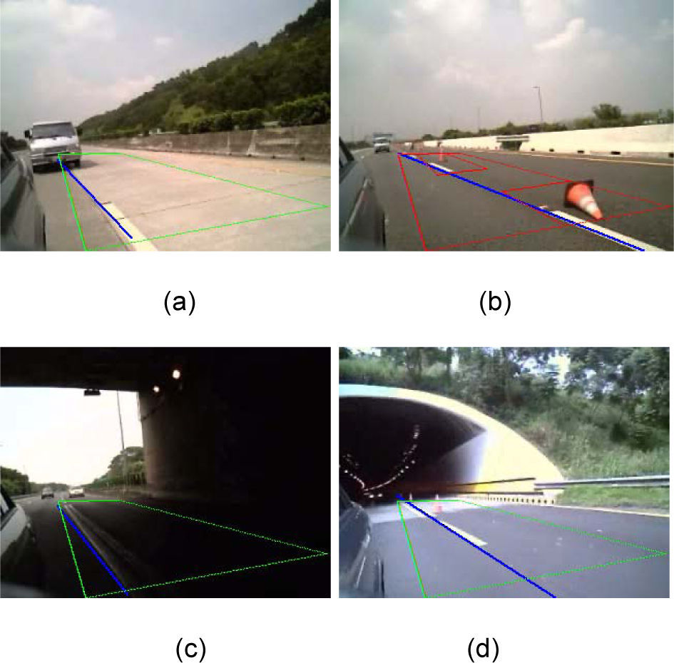
The practical programming interface is shown in Figure 8. The system tracks lateral vehicles and marks adjacent lane line at the same time. The green-line rectangle is the ROI for lateral vehicle detection. When the vehicle entered this region, the color of the line turns red. The blue line is the detected lane line, and the distances of the lateral vehicles located within the ROI are shown at the right side of the window. Moreover, the current driving lane and the driving state are shown at the lower right corner of the window.

Figure 9 shows the detection results for different road conditions: (a) the neighboring lane with newly paved asphalt of different colors, (b) traffic cones laying on the neighboring lane, (c) vehicle driving into the tunnel, and (d) vehicle driving out of the tunnel. In these conditions, the results of lane line detection are favorable.

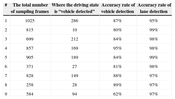
To prove the validity of our method, we captured the images of detection result every ten frames, and investigate these images one by one. In this experiment, there are 9 video sequences used to capture the images when the vehicle is driving on Taiwan’s highways. Table 3 tabulates the accuracy rates of the proposed lane and vehicle detection methods. The accurate rate of vehicle detection is defined as the rate that the vehicle is located correctly when the system is in “Vehicle Detected” state. The results prove that the system is well performed. But, the vehicle detection rate of video 9 is very low, the reason is that only a small portion of the lateral vehicle is located in the detection area and the elapsed time within this area is very short.
Accuracy rates of the lane detection and vehicle detection.
| # | The total number of sampling frames | Where the driving state is “vehicle detected” | Accuracy rate of vehicle detection | Accuracy rate of lane detection |
|---|---|---|---|---|
| 1 | 1025 | 286 | 87% | 95% |
| 2 | 815 | 10 | 80% | 99% |
| 3 | 699 | 212 | 84% | 98% |
| 4 | 857 | 169 | 95% | 98% |
| 5 | 905 | 189 | 84% | 99% |
| 6 | 371 | 27 | 81% | 98% |
| 7 | 828 | 149 | 88% | 97% |
| 8 | 258 | 28 | 89% | 97% |
| 9 | 584 | 94 | 62% | 97% |
In this paper, we propose a new driver assistance system based on image processing techniques. The system provides the abilities of lane detection, vehicle detection, and distance measurement for lateral vehicle. Experimental results show its robustness in the cases of complex environment conditions.