


This paper addresses a vehicle scheduling problem encountered in the cold chain logistics of the frozen food delivery industry. Unlike the single product delivery scenario, we propose an optimization model that manages the delivery of a variety of products. In this scenario, a set of customers make requests for a variety of frozen foods which are being loaded together. The objective is to find the routes that represent the minimum delivery cost for a fleet of identical vehicles that, departing from a depot, visiting all customers only once and returning to the depot. The delivery cost includes the transportation cost, the cost of refrigeration, the penalty cost and cargo damage cost based on the characteristics of different frozen food products. Apart from the usual constraints of time windows and loading weight, the study also takes into account the constraints of loading volume related to the unit volume of different frozen foods. We then propose a Genetic Algorithm (GA) method for the model. Computational tests with real data from a case validate the feasibility and rationality of the model and show the efficient combinations of parameter values of the GA method.
The need for fresh, refrigerated and frozen food has grown continuously in recent years due to high demand for healthy and convenient diets in urban fast-paced daily living. Correspondingly, the market for low-temperature logistics is expanding due to demand for low-temperature food [1]. This paper considers a specific vehicle routing problem in the cold chain distribution industry for a variety of frozen food products. Compared to normal temperature distribution, cold chain distribution requires strict temperature and time control to preserve food quality. Frozen food products with low thermal inertia (such as ice cream) are more vulnerable to any disruption in the cold chain distribution process. As frozen food distribution companies tend to serve rather large numbers of customers in dispersed locations, it is crucial for them to design the routes for vehicles in an efficient way so as to minimize the delivery cost while maintaining or even improving food and service quality for customers.
In the past, most studies on the vehicle routing problem (VRP) have focused on the expansion of the network and algorithms [2,7,10-13,16-18]. Little attention has been paid to the improvement of the vehicle routing model [3]. The optimization models used for vehicle routing problems in current cold chain distribution studies often aim to minimize the total delivery cost, comprising the transportation cost, energy cost and deterioration cost [4-7]. Also, until now, vehicle routing models have been built for a single product only and the constraints considered in the model and its variants have always been the loading weight and time windows [4-9]. However, as is widely recognized, the reality is that customer orders are not limited to a single frozen food product and different frozen food products ordered by one customer are often loaded together in one vehicle.
The factors considered in this scenario include unit volume, price, the punishment degree and perishable coefficient of different frozen food products.
In addition to the usual constraints of time windows and the loading weight, the volume capacity of the vehicle is also taken into consideration.
This paper proposes a solution to the VRP in multi-product frozen food distribution taking into account the multiple factors discussed above.
The reminder of this paper is organized as follows. Section 2 describes in detail the model development process. In Section 3, the GA approach for the distribution model is proposed. Section 4 applies the GA in a case study. Finally, conclusions and future research are presented in Section 5.
2The routing model for frozen food distribution2.1Assumptions and constraintsAssuming a fleet of identical vehicles with given internal and external dimensions of length, width and height, the objective is to find a set of minimum cost vehicle routes, starting from and terminating at the depot, such that:
- 1)
The depot centre houses a fleet of identical vehicles with a fixed rate υ.
- 2)
The loading weight and volume of the vehicle are known and there is no midway assignment.
- 3)
The geographic locations and time windows of customers are known.
- 4)
Information concerning the mass and loading volume of per unit frozen food products is given.
- 5)
Each customer’s orders are delivered by exactly one vehicle during distribution, but each vehicle can serve different customers.
- 6)
The vehicle maintains a constant temperature inside and outside during distribution.
- 7)
The cumulate weight and volume of a vehicle k (k = 1,2...K) does not exceed its capacity M and N at any point on the route.
- 1)
The cargo damage cost of frozen food
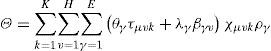
The main damage cost in the process of distribution consists of two parts: a) damage cost accumulated due to transit time, b) damage cost caused by a break in the cold chain during a series of links including the arrival of food, code inspection and shelving. We assume that the quality of the frozen food in the transportation process and customer service process is inversely proportional to the time and the demand of customers, respectively. Hence, considering different damage rates and the price of frozen food products, the cargo damage cost © can be expressed by Eq. 1 [4].
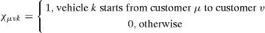
where θγ denotes the cargo damage rate of the frozen food γ (γ = 1,2...E) during the process of transportation, λγ is the cargo damage rate of the frozen food γ during customer service, ργ represents the unit price of the frozen food γ, τμvk indicates the time of vehicle k from customer μ to customer v, βγv is the order of food γ from customer v. The (routing) decision variable χμvk is defined as
- 2)
The vehicle transportation cost
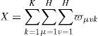
The transportation cost includes fuel consumption, vehicle maintenance, etc. And the cost is generally proportional to the distance [7]. The transportation cost is given by:
where ϖμvk denotes the transportation cost of vehicle k between customer μ and v.
- 3)
The refrigeration cost
The refrigeration cost relates mainly to two aspects. One is heat transfer inside and outside the refrigerator caused by the temperature difference during transportation. On the other hand, heat will exchange during loading/unloading process because of air convection. The refrigeration cost can be obtained by calculating the cost of the refrigerant consumed. Consumption of the refrigerant is related to the heat transfer coefficient, the surface area of the vehicle, the outside temperature, stored-product temperature and other factors.
- a)
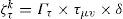
The thermal load Гτ due to the difference in temperature can be obtained using the following formula [8]:
where ξ denotes thermal conductivity, ΔT is the temperature difference. The average area of the vehicle Σ=ΣωΣv, α is the depreciation degree of the vehicle, ∑ω indicates the external surface area and ∑v the internal surface area
The cost of vehicle k from customer μ to customer v is shown as follows:
where δ denotes the unit cost of refrigerant, τμv represents the time from customer μ to customer v. The cooling cost of refrigerator during transportation can be expressed as follows:
- b)
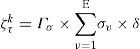
With reference to the literature [9], the vehicle thermal load during loading/unloading can be obtained using the specific formula:
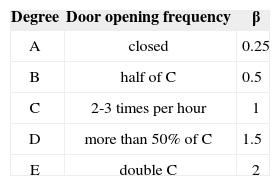
where β is related to door opening frequency. Its value is shown in Table 1.
Thus, the cooling cost of vehicle k at customer v is
where σv is the service time at customer v. The cost of refrigeration during loading can be expressed by
The total energy consumption cost Λ is the sum of Λ1 and Λ2
- a)
- 4)
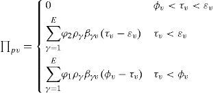
The penalty cost of customers
This research adopts the time windows constraint, which allows for arrival at a time outside the window with a penalty. If the service at customer starts inside the time window [ϕv,εv], no penalty is incurred. If a vehicle starts servicing customer before time ϕv or after time εv, a penalty has to be paid. The penalty cost is proportional to the value through non-negative weights φ1 and φ2, respectively. This study constructed the penalty cost function of time windows during the distribution of a variety of frozen food products. Assuming that the penalty cost is correlated to the price of different frozen food products and the exceeded time, it can be formulated as follows:
where τv is the time of arrival at customer v, φ1 is the penalty coefficient for being early, φ2 is the penalty coefficient for being late. The weight for delayed delivery at customers is set to be larger than that for early delivery (i.e.φ1> φ2), and the weights for each customer can be adjusted accordingly.


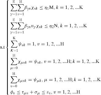
where η1 and η2 represent the utilization rate of the loading weight and loading volume, respectively. vγ is the unit volume of frozen food γ.
The (routing) decision variable χvk is defined as
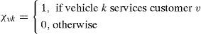
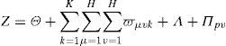
In this model, the objective function (11) aims to minimize the total cost for the vehicles to visit all customers, constraint (12) and constraint (13) ensure that the loading weight and loading volume of each vehicle is not exceeded, equation (14) ensures that each customer is served by only one vehicle, equations (15) and (16) guarantee that each customer is visited exactly once, and equation (17) is the constraint of time windows.
3Solution approachThere are two types of algorithms for solving the VRP. One is the exact algorithm and the other is the heuristic algorithm. The exact algorithm includes the branch and bound method, the cutting plane method, the network flow algorithm, dynamic programming, etc [10]. As the complexity of the solution for the VRP is NP-hard, the exact solution can only be used to solve a VRP with a small number of distribution points [11].
In contrast, many heuristic algorithms, such as the genetic algorithm (GA) [12-13], hybrid genetic algorithm [14] and particle swarm optimization algorithm [15], have been used widely in a variety of combination optimization problems. Existing literature that compares different algorithms for VRP has demonstrated the superiority of the GA as it can handle greater problems with less computational effort [12-13]. However, the quality of the convergence process in GA depends on the specific choices of strategies and combinations of operators or parameter values [16]. As stated above, the vehicle scheduling problem for distribution companies in frozen food delivery is considerable. Thus, this paper proposes the use of a GA to address the problem and gives a detailed description of the operators.
3.1The implementation of the genetic algorithmGA simulates the survival of the fittest among individuals over consecutive generations throughout the solution of a problem.
Each generation consists of a population of character strings that are analogous to the chromosomes. Each individual represents a point in the search space.
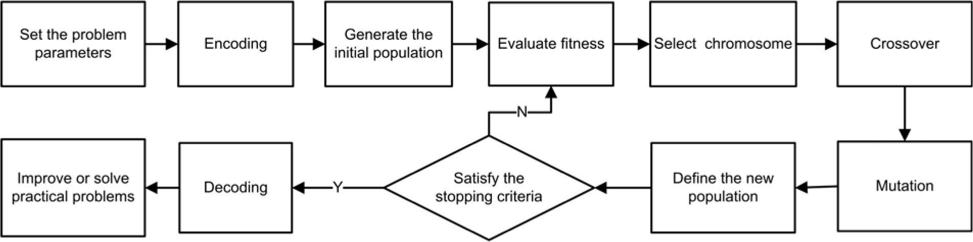
The individuals in the population are then exposed to the process of evolution. Genes from good individuals propagate throughout the population, thus making successive generation become more suited to its environment [21]. The overall structure of the GA is illustrated in Figure 1.

Step 1: Set the initial values of loading weight, loading volume, population size, number of iterations, crossover probability and mutation probability.
Step 2: Generate an initial population T of chromosomes for which each chromosome represents a feasible route.
Step 3: Evaluate each chromosome using the fitness function.
Step 4: Select the chromosomes the fitness of which meet the specified requirements according to the selection operator.
Step 5: Cross over two chromosomes (τi,τj) using the crossover operator, with crossover probability ω3.
Step 6: Chromosome τ is designed to mutate according to the mutation operator once it meets the condition sτ,≥ω2where sτ is a parameter randomly sampled in the range [0,1] and ω2 is the mutation probability, otherwise no variation.
Step 7: The GA is implemented with the stopping criteria: the maximum number of iterations and maximum number of iterations without improvement.
3.2Genetic algorithm design notesIn this paper, the chromosome is a permutation of the integer of all customers (1,2,..., H) that place an order for frozen food on separate routes.
This section is devoted to the detailed presentation of the coding method design, fitness evaluation, generation of initial solutions, selection, crossover and the mutation operator.
- 1)
Design of coding method
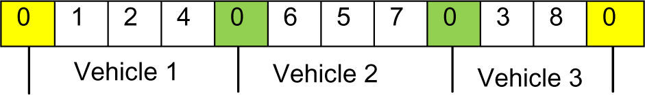
The distribution centre with K vehicles determines the number of distribution routes. Add K-1 virtual distribution centres which are represented by 0 to reflect the routing problem of vehicle in the coding.
Figure 2 depicts an example of a chromosome comprising eight customers serviced by three vehicles.
- 2)
Generation of the initial population
First, generate the permutation of H customers using the randperm function. The first and the last numbers of the permutation are set to 0 to represent that the vehicle starts from the yard and eventually returns. Then, insert virtual distribution according to vehicle loading weight M and loading volume N, and so forth until the population number is met.
During the process, chromosomes with the same fitness as another are replaced by the new random population to ensure the diversity of the population.
- 3)
The fitness evaluation
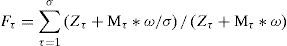
The corresponding distribution routing scheme of chromosome τ (τ = 1,2,...,σ) is preferred for two reason: (i) it satisfies the constraints of the problem and (ii) the value of the objective function z in the routing optimization model is smaller. In this model, the coding design and the generation of the initial population can meet the constraint conditions: (a) each customer receives a delivery service and (b) each customer is served by one vehicle. Each path of the chromosome is judged by the constraints of vehicle loading weight and loading volume one by one. If the number of infeasible paths of chromosome τ is Mτ (Mτ = 0 denotes that chromosome τ is a feasible solution), the objective function value is Zτ and the fitness evaluation of chromosome τ is Fτ determined by the following formula [17]:
In the formula, assume that ω = 1000 is the penalty weight assigned to each infeasible path. The equation guarantees that the chromosome with the lower distribution cost can obtain a higher fitness evaluation.
- 4)
Selection operator design
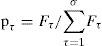
Based on the roulette wheel selection method (RWS) [11] in which the probability of a chromosome participating in a crossover is directly proportional to its relative fitness:
Then accumulated normalized fitness values are computed.
The selected individual is the first one the accumulated normalized value of which is greater than ς, which is a random number sampled in the range [0,1] to guarantee the optimal individual can be reserved to the next generation.
- 5)
Crossover operator design
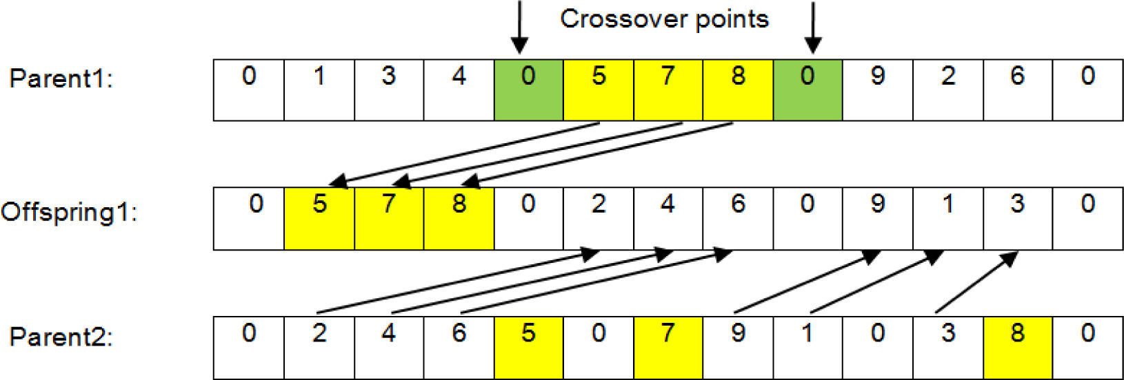
The vehicle routing problem with time windows (VRPTW) is characterized by randomness between groups and orderliness within the group. The general crossover operator will destroy the excellent substring, so we use an efficient crossover operator based on the traditional one-point crossover (1px) operator [19]. In this operator, two virtual distribution points of one chromosome are selected.
If n is the number of routes in a chromosome, there are n+1 crossover points. Each of these points is selected with equal probability.
Customers on the chosen route are inherited by the offspring from the parent and the other customers are placed in the order in which they appeared in the other parent. After exchanging the roles of the parents, the same procedures are employed to produce the second descendants. Figure 3 is an illustrative example of the crossover operator.
- 6)
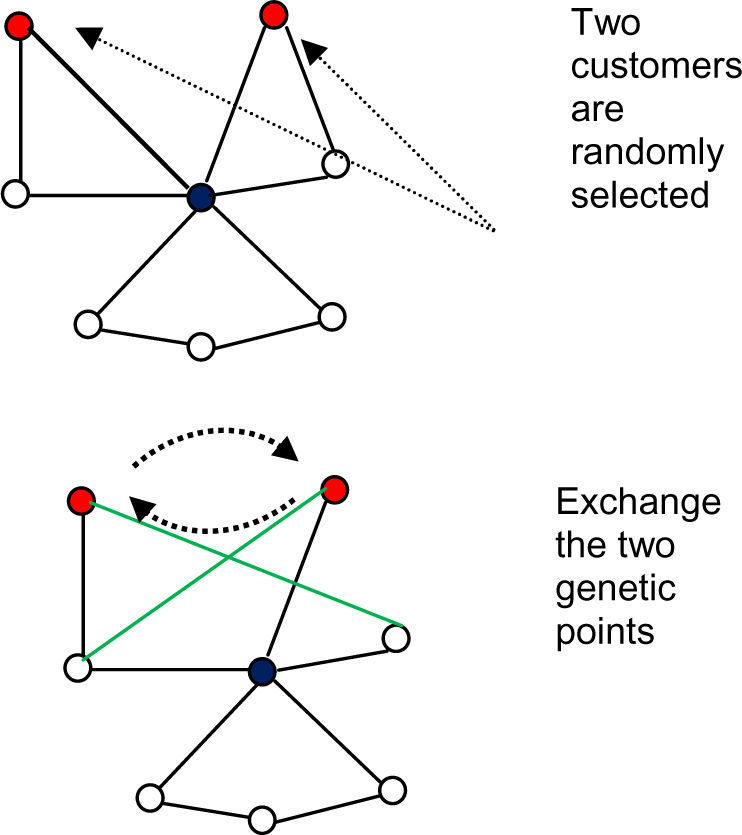
Mutation design
The possibility of chromosome variation is relatively small and it plays an auxiliary function in the GA. We propose a 2-exchange mutation operator. As shown in Figure 4, two genetic points on the chromosome, other than the distribution centres, are randomly selected for exchange.


For our computational experiments, we turn to an instance built using actual data from a company working in Beijing. It is a cold chain logistics company with a distribution network covering all districts and counties in Beijing. Each trip starts and ends at the distribution centre. The company has approximately 400 stations and five time periods.
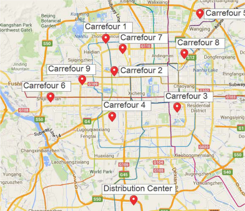
To introduce the steps of GA method for the proposed vehicle routing model, we constructed a smaller instance by reducing the number of stations and focusing on the period from 3:00 am to 8:00 am. We chose nine large Carrefour stores in Beijing as the customers, as shown in Figure 5.

Usually, the suggested storage temperature of frozen food products is below -18°C, in which microbial growth is completely stopped, and both enzymatic and non enzymatic changes continue but at much slower rates during frozen food shelf life [20].
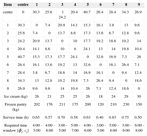
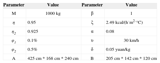
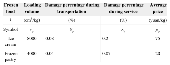
We assume that the average temperature outside is 20°C and the temperature difference will stay at 38°C. The assumptions concerning customer locations (Table 2), vehicles (Table 3), and frozen product information (Table 4) are based on the results of a survey.
Distance between the delivery centre and customer, requirement for frozen food products and time constraints.
| Item | centre | 1 | 2 | 3 | 4 | 5 | 6 | 7 | 8 | 9 |
|---|---|---|---|---|---|---|---|---|---|---|
| centre | 0 | 30.3 | 25.6 | 1 24.2 | 20.4 | 40.7 | 26.4 | 28.4 | 34.3 | 26.9 |
| 1 | 30.3 | 0 | 7.4 | 20.9 | 14.1 | 15.3 | 16.1 | 3.8 | 13 | 9.6 |
| 2 | 25.6 | 7.4 | 0 | 13.7 | 8.6 | 17.3 | 13.6 | 6.7 | 12.8 | 9.6 |
| 3 | 24.2 | 20.9 | 13.7 | 0 | 10 | 17.7 | 19.2 | 18.6 | 10.2 | 14 |
| 4 | 20.4 | 14.1 | 8.6 | 10 | 0 | 24.1 | 13 | 14 | 19.8 | 10.4 |
| 5 | 40.7 | 15.3 | 17.3 | 17.7 | 24.1 | 0 | 32.6 | 16.9 | 7.3 | 26 |
| 6 | 26.4 | 16.1 | 13.6 | 19.2 | 13 | 32.6 | 0 | 16.1 | 26.4 | 7.1 |
| 7 | 28.4 | 3.8 | 6.7 | 18.6 | 14 | 16.9 | 16.1 | 0 | 9.4 | 12.4 |
| 8 | 34.3 | 13 | 12.8 | 10.2 | 19.8 | 7.3 | 26.4 | 9.4 | 0 | 18.6 |
| 9 | 26.9 | 9.6 | 9.6 | 14 | 10.4 | 26 | 7.1 | 12.4 | 18.6 | 0 |
| Ice cream (kg) | 26 | 21 | 25 | 25 | 26 | 18 | 24 | 29 | 30 | |
| Frozen pastry (kg) | 202 | 176 | 211 | 175 | 200 | 120 | 210 | 230 | 150 | |
| Service time (h) | 0.65 | 0.57 | 0.70 | 0.58 | 0.63 | 0.40 | 0.83 | 0.75 | 0.50 | |
| Required time window [ϕv, εv] | 4:00 - 5:00 | 4:00 - 6:00 | 3:00 - 5:00 | 5:00 - 7:00 | 4:00 - 6:00 | 3:00 - 5:00 | 5:00 - 8:00 | 3:00 - 6:00 | 6:00 - 8:00 | |
As our problem is highly combinatorial, the performance of the GA strongly depends on its parameterization [21]. This section reports the results of computational experiments for different parameter combinations to determine the optimal GA parameter settings.
All the algorithms previously described in this paper are implemented in Matlab. The GA is carried out on a 2.09 GHz Intel CPU in Microsoft Windows XP. The main aim of the experiment is to determine the optimal GA parameter settings to obtain the best algorithm performance. For this purpose, we tried different GA parameters including the population size ω1, the mutation probability ω2 and the crossover probability ω3 to determine the distribution cost. The results, summarized in Figures 6-7, were obtained from 10 independent runs for different parameter combinations.
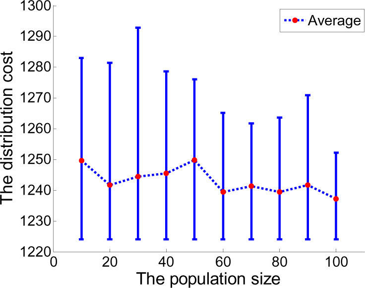
Figure 6 shows us the best, worst and average routing costs among the 10 runs of GA with ω2 = 0.02, ω3 = 0.7 and different population sizes for instance. The results show that the GA method with a discrete population size from 10 to 100 can always find the best solution within 10 runs. Furthermore, the worst and average values are relatively small, especially when ω1 ∈ [60-100]. It is a testament to the impact of the GA method that global searching ability increases with increased population size [22].

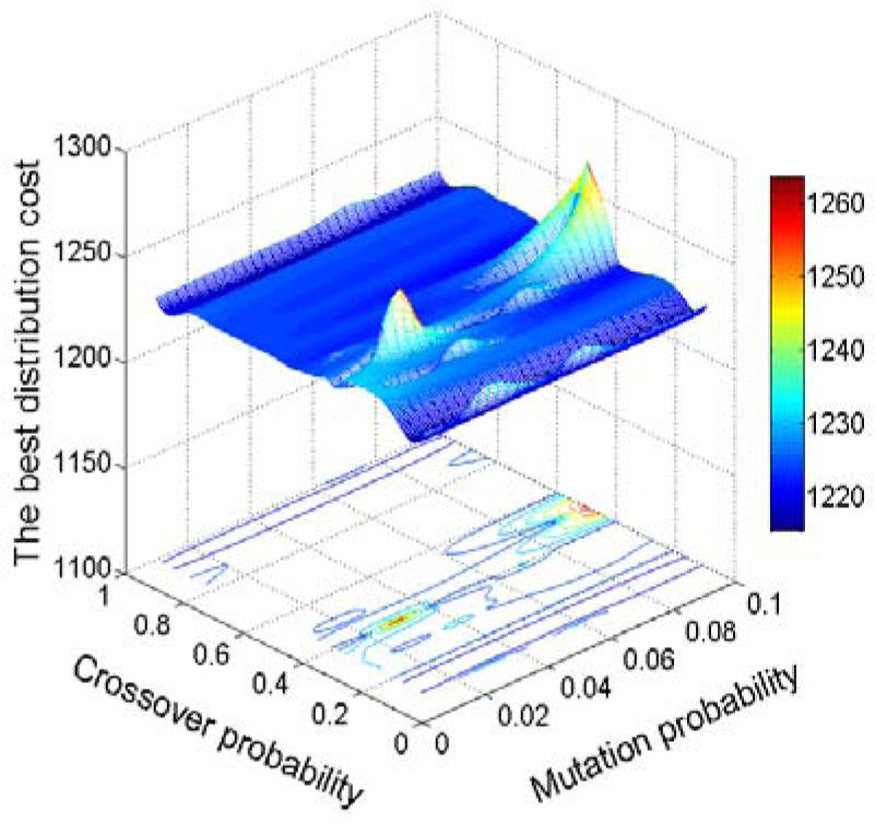
In Figure 7, the behaviours for different combinations of mutation probability and crossover probability are given. Behaviour is defined as the best distribution cost among 10 runs of each combination. The experimental data in the above surface chart come from 1000 combinations with a population size ω1 = 60, the mutation probability ω2 ∈ [0.01-0.1] and crossover probability c3 e [0.1-1]. The results show that the GA with crossover probability ω3 ∈ [0.5-0.9] and mutation probability ω2 ∈ [0.02-0.09] can always find the best distribution cost, as seen in Figure 7. However, the results with crossover probability ω3 ∈ [0.1-0.4] and mutation probability ω2 ∈ [0.01-0.04] ∪ [0.07-0.1] for the model are unsatisfactory.
4.3Analysis of results
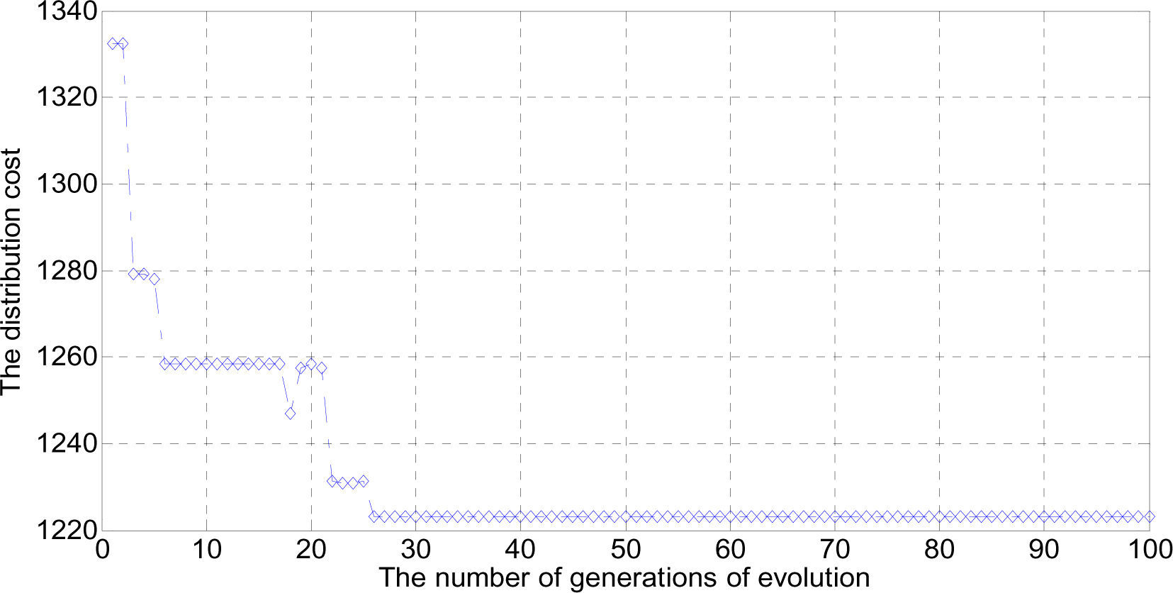
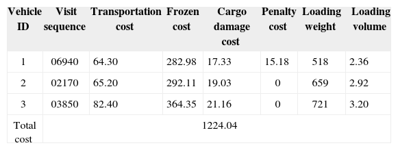
In this subsection, the total routing cost of 100 iterations obtained from the GA when ω1 = 60, ω2 = 0.09 and ω3 = 0.6 is shown in Figure 8. The distribution cost decreases with increasing iterations until reaching the best solution of 1224.04 which operates 74 iterations without improvement. The results represent the convergence characteristics of GA for the case.

Detailed information on the optimal chromosome is shown in Table 5. According to the result, the distribution centre needs three vehicles to complete the delivery work. The best distribution program is as follows: the route for vehicle 1 is 0-69-4-0, the route for vehicle 2 is 0-2-1-7-0 and the route for vehicle 3 is 0-3-8-5-0. The transportation cost, frozen cost and cargo damage cost of the three vehicles are comparable. From the perspective of the vehicle utilization, there is no phenomenon of excessive overloading, which is in favour of vehicle maintenance. Except for the penalty cost of waiting in the case of vehicle 1, the remaining vehicles can serve the customers within their time windows. Overall, the proposed model can provide distribution companies with a reasonable and practical vehicle scheduling program, thereby saving costs, maintaining food quality and improving customer satisfaction.
5Conclusions and future researchThis paper investigates a unique vehicle routing problem in the frozen food distribution industry taking into account various factors. The problem is of interest because of its theoretical complexity and the important practical applications in cold chain distribution. We formulate the problem into one optimization model with the objective of minimizing the total cost (including transportation cost, refrigeration cost, penalty cost and cargo damage cost) based on a real scenario. We also propose one heuristic, genetic algorithm, to solve this problem. As this problem is unique and no benchmark exists, experiments have been conducted using an example case. The case was designed based on actual information in a frozen food distribution company to verify the rationality and the feasibility of the model in improving the efficiency of transport while ensuring the food fresh and safe. In general, we find that the GA method can provide sound solutions with good robustness and convergence characteristics in a reasonable time span.
The focus of our future studies in this area will be to increase the complexities of assumptions to make them closer to the real world. For example, some constraints commonly used in container loading research, such as the loading-bearing strength of the boxes and vertical stability of the foods, can be used in the vehicle routing problem for frozen food delivery [23]. There are also factors that are common but not known in advance in real-world cold chain distribution, such as the travel time of vehicle, service time for customers and customers’ different delivery requirements. Other factors include fleet size, mixed-type vehicles, multi-temperature joint distribution and vehicle routing problems with backhauls, etc.
These factors have a considerable impact on system performance. Thus, research on vehicle scheduling problems in frozen food distribution including these factors is of great interest and importance.
This research was funded by the Lab of Logistics Management and Technology, School of Economics and Management, Beijing Jiaotong University.