


This paper treats the estimation of the state of a nonlinear system with unknown input. The nonlinear system is described by a multimodel with unknown function of activation but depending only on the state. The method of design of the multiobserver is described by using the second method of Lyapunov and their candidate functions. The sufficient obtained stability conditions are expressed in terms of Linear Matrix Inequalities (LMI) and are obtained first using the Lyapunov quadratic functions and secondly by using Lyapunov polyquadratic functions. This latter technique seems to be less conservative and less constraining than the first. Illustrative examples are presented in this paper.
Este artículo trata la estimación de estado de un sistema no lineal con una entrada desconocida. El sistema no lineal se describe por un multi-modelo con una función desconocida de activación, pero dependiendo sólo en su estado. El método de diseño del multi-observador se detalla mediante el segundo método de Lyapunov y sus funciones candidatos. Las condiciones de estabilidad obtenidos se expresan en términos de desigualdades matriciales lineales (LMI) y se obtienen de la utilización de las funciones cuadráticas de Lyapunov en un primer estudio y de las funciones poli cuadráticas de Lyapunov en un segundo estudio que aparece menos conservador y menos restrictivo que el primero. Múltiples ejemplos ilustrativos se presentan en este documento.
A system is often controlled simultaneously by known and unknown inputs. The measurements taken at output of the system do not give complete information about the internal states, because a part of these states is not directly measurable. Moreover, not for purely technological reasons, but also for cost reasons, the number of sensors is limited.
So the idea, for several years, has been the replacement of the material sensors by software or state observers, which make possible the rebuild of internal information (states, unknown inputs, unknown parameters) using, only, the known inputs and the measured outputs [18,19,20,21].
The need of internal information can be used for: identification, command by feedback control, monitoring and diagnosis of the system. The problem of the design of observers is in the heart of the general control problem [15,16].
Among the solutions brought to the problem of the state and output estimation of in the presence of unknown inputs, two approaches of developing multiobserver emerged. The first one supposes an a priori knowledge of information about these not measurable inputs; in particular, the filter of Kalman who allows to rebuild the state of the system in the presence of measurement noises which are defined like unknown inputs, by using a priori statistical knowledge on these noises. The second approach proceeds either by estimation of the unknown inputs or by their complete elimination from the equations of the system [1, 2, 3, 5, 8, 23, 24, 28]. The observers with unknown inputs have attracted the attention of many researchers like Abdelkader Akhenak [1, 2] who used unknown input observers to detect and isolate sensor faults in a turbofan engine.
The crucial problem in the synthesis of the observers with unknown inputs is the convergence of the estimation error towards zero. Several works used the second method of Lyapunov and their quadratic functions for the stabilization of the estimation error in the case of linear systems [4, 6, 7, 9, 10, and 11] and in the case of nonlinear systems.
However, this method generates very conservative conditions of stability of the observer in particular for certain classes of nonlinear systems such as the hybrid dynamic systems [27], the saturated systems and linear piecewise systems, where there is no information about space state partition’s [25]. Whereas, the use of the non quadratic Lyapunov functions like the polyquadratic functions and the continuous piecewise functions, allows the reduction of the conservatism of the quadratic method and results are often less pessimistic for the stabilization and the control of the systems [9].
For this reason, it is interesting to use the polyquadratic Lyapunov functions for the stabilization of the error estimation in the case of a nonlinear multiobserver with unknown inputs which is used for the diagnosis and the supervision of a nonlinear systems described by a multimodels [1].
This paper is divided into five parts:
After the introduction, the second part presents the multimodel approach and describes the conditions for stabilizing a nonlinear system described using this approach.
The third part explains how to build a multiobservers and ensure its convergence.
The fourth part deals with the assessment and determination of the unknown input of the system.
Three examples are described in this paper to illustrate the power of the proposed method.
Notation: Throughout the study, the following useful notations are used:
(X)T = the transpose of the matrix X
(Y)−1 = the inverse of the matrix Y
(Z)− = the pseudo inverse of the matrix Z
l= the n × n identity matrix
2Multimodel Approach
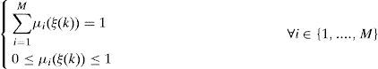
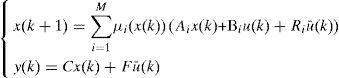
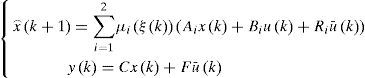
The multimodel approach makes possible the modeling of nonlinear system behavior by using several local linear models. Each local model contributes to this total representation according to its weight function μi(ξ(k)) with values in the interval [0, 1]. The multimodel structure is described as follows [1]:
with:
Where x(k) Rn is the state vector, u(k) Rm is the vector of the known inputs, Rq is the vector of unknown inputs and y(k) Rp represents the vector of measurable outputs.
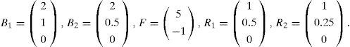
For the ith local model, Ai∈ Rn×n is the state matrix, Bi∈ Rn×m isthe matrix of input, Ri∈ Rn×q is the matrix of influence of the unknown inputs on the state x(k), F∈ Rp×q the matrix of influence of the unknown inputs on the output y(k) with rank(F)=q and C∈Rp×n is the matrix of output. Finally, ξ(k)represents the vector of decision depending on the input and/or the measurable state variables. At every moment, μi(ξ(k))indicates the degree of activation of each local model in the global model. Choosing the number M of local models of this multimodel can be intuitively achieved with taking into account the number of functioning modes observed [10]. However, determining the matrices Ai, Bi, Ri and Di needs the use of adapted estimation parametric techniques [10] or techniques of linearization [12,13].
The analysis and the synthesis of such systems can be made by adopting some tools of the linear field. One finds for example in [26 and 27] which is inspired directly from the use of linear systems stability tools for the analysis of the stability and stabilization of nonlinear systems. In [17, 18 and 20], the author deals with the problem of the estimation of state of nonlinear systems described by multimodels, and made it possible by designing observers, for the generation of defects. However, in all this work, the authors suppose that the variable of decision ξ(k) is measurable depending on u(k) or/and y(k) [1, 2 and 3]. In the problem of the diagnosis, this assumption obliges to design banks of observers containing multimodel in which the functions of activation depends on the input u(k), for the detection and the localization of the defected sensors, or on the output y(k) for the detection and the localization of the defects actuators. This strategy requires the development of two different multimodels, representing the same system. To overcome this problem, it is interesting to consider the case where the functions of activation depend on the state of the system. Among rare public works in this context, we can cite for example [25] which, under the assumption of Lipschitzian activation functions μi(ξ (k)), propose an observer of the Luenberger type. The stability conditions of this last assumption are formulated in the form of Linear Matrix inequalities (LMI) easy to solve.
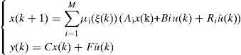
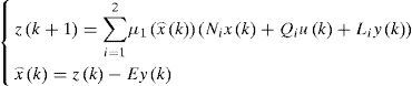
3Design of multiobserver with unknown inputs3.1General structure of the multiobserverIn this section, we consider a nonlinear discrete time system described by a multimodel using activation functions depending on the state of the system:
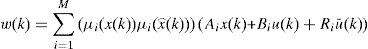
It is supposed that the number of unknown entries is lower than the number of measured outputs. The multimodel with non-measurable decision variables (3) can be written as follows:
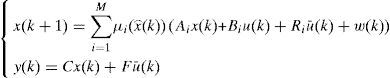
Where:
The multimodels (3) and (4) are equivalent. For the design of the observer, we will use the second structure.
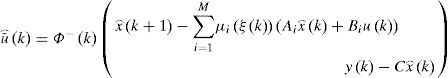
The multiobserver is taken in the form:
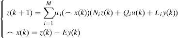
Where Ni,∈Rn×n,Qi, ∈Rn×m, Li∈Rn×p and E are the gain matrices of the ith local observer with unknown input.
The variable z(k) is an intermediate variable allowing to deduce the value estimated from the state x⌢k.
Obviously, the observer uses only the known variables u(k) and y(k), u¯k being not measured.
The whole of these matrices must be given with a high degree of accuracy from a numerical point of view in order to guarantee the convergence of the state estimated by the observer towards the real state. For that, let us define the state estimation error:
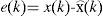
Starting from this definition and by using the expression of x⌢k given by the equation (6), the expression of the error becomes:

with:

Then, we can express the temporal evolution of the state error in order to analyze its convergence towards zero.
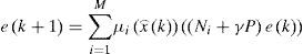
Thus, at time (k + 1), the state estimation error is expressed as follows:
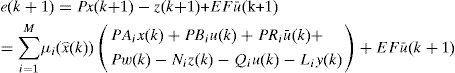
After recognizing the terms at the right side of equation (10), and by using the definitions of y(k) and z(k), (10) becomes:
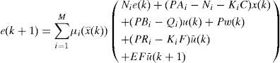
with:
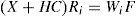
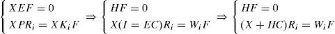
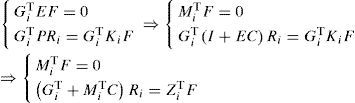
If the following conditions are satisfied:


then, the dynamic of the state estimation error becomes:
It is clear that the above dynamic is disturbed by w(k). To synthesize the matrix of the multiobserver (6), two approaches are proposed in the following subsections.
3.2Global convergence of the multiobserverFor the stabilization of the dynamic error (14), we propose two approaches which are based on two types of quadratic and polyquadratic Lyapunov functions.
Hypothesis: It is supposed that term w(k) defined in (5) satisfied the following conditions:
Where γ is a positive constant of Lipschitz.
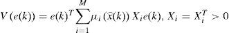
3.2.1Global convergence of the multiobserver by the quadratic approachIn this part, the stabilization of the dynamic error (14) is based on a quadratic Lyapunov function of the form:
Proposition 1:
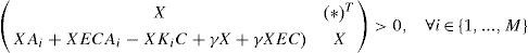
The state estimation error between the multimodel (4) and the unknown input multiobserver (6) converges globally asymptotically towards zero if there exists matrices X = XT > 0, H and Wi such that the following conditions are hold ∀i∈1,...,M:
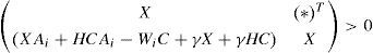

Multiobserver (6) is then completely defined by
Proof.


The variation of the quadratic function (16) on all the trajectory of the multimodel (4) is:

By using the equations (14) and (16), ∆V(e(k)) can be written as follows:
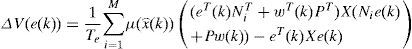
According to the condition of Lipchitz (15), ∆V(e(k)) becomes:
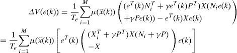
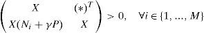
Since the functions of activation are verifying the conditions of convexity (2), the variation of the quadratic function (16) is negative if:

The use of equation (22), the hypothesis X=XT>0 and the Schur complement leads to:
Using equations (9) and (13b), the above inequality (23) becomes:
However, expression (24) is a bilinear matrix inequality BMI with synthesis variables X, E and Kj. In order to convert these conditions into an LMI formulation, we consider the following changes of variables:


Using the new variables of equations (25) and (26), inequality (24) becomes:
The two equality constraints (17b) and (13c) are obtained by pre-multiplying the last two constraints (13a) and (13d) by X = XT > 0 with the change of variable (25) and (26):
Therefore classical numerical tools may be used to solve LMI problem (17a) subject to linear equality constraints (17b) and (17c).
After having solved this problem, the different gain matrices Ni, Li, Qi, and E defining the multiobserver (6) can be deduced from the knowledge of X, H and Wi as given in equations (18). This completes the proof.
3.2.2Determination techniques of the multiobserver gainsTo determine gain matrices of the multiobserver (6) by quadratic approach, we propose to follow an algorithm with the following steps below:
Step 1:determination of the matrices X, H and Wi∀i∈1,...,M.
We solve the Linear Matrix Inequalities (17a) in synthesis variables X, H and Wi subject to linear equality constraints (17b) and (17c). This problem can be solved by LMITOOL of Scilab.
Step 2:determination of the gains matrices Ni, Li, Qi, and ∀i∈1,...,M.
After the knowledge of the matrices X, H, and Wi, we determine the other gains matrices of equations (18) defining the multiobserver (4).
Remark 1:although the quadratic approach makes synthesis possible by ensuring the convergence of multiobserver (6) towards the multimodel (4), it constitutes in certain cases a source of conservatism due to the search of a unique matrix X which stabilizes a significant number of local observers. Also, researchers [25] define three cases where the quadratic approach shows conservative:
- -
Case of the saturated systems,
- -
Case of the piecewise linear systems,
- -
Case of the multimodels with high number of local models
These last points become the principal objectives of the stability study of by using the polyquadratic approach.
3.2.2.1Global convergence of the multiobserver by the polyquadratic approachIn this part, the stabilization of the dynamic error (11) is based on a polyquadratic Lyapunov function of the form:
Where (Xi, i = 1,...,M) are symmetric positive definite matrices.
That is to say the following system:
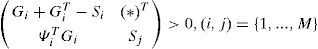
Theorem 1[7]: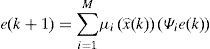
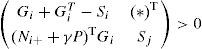
System (29) is polyquadratically stable if and only if there exist symmetric positive definite matrices Si, Sj and matrices Gi of appropriate dimensions such that:
The goal of this second approach is to mitigate the conservatism of the quadratic approach by formulating new less constraining conditions of stabilization of the dynamic error (14) by using theorem 1:
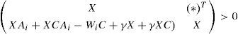
Proposition 2:The state estimation error between the multimodel (4) and the unknown input multiobserver (6) converges globally asymptotically towards zero if there exist symmetric positive definite matrices Si and matrices Mi, Zi, and Gi, of appropriate dimensions such that the following conditions hold ∀(i,j)∈1,...,M:
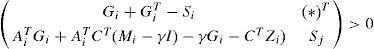

Multiobserver (6) is then completely defined by
Proof.


According to the hypothesis (15) the estimation error (14) can be written as follows:
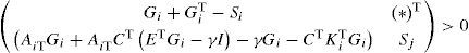
By substituting matrix Ψi,. by the matrix (Ni + γP) in inequality (30) of theorem 1, one obtains the following condition, (i, j) = {1,...,M}:
Using equations (9) and (13b), the inequality (35) becomes:


Using the new variables of equations (36) and (37), inequality (35) becomes:
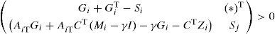
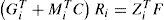
The two equality constraints (32a) and (32b) are obtained by pre-multiplying the last two constraints (13a) and (13d) by GiT with the change of variable (37) and (38):
Therefore classical numerical tools may be used to solve LMI problem (31) subject to linear equality constraints (32a) and (32b). After having solved this problem, the different gain matrices Ni, Li, Qi, and E defining the multiobserver (2) can be deduced from the knowledge of Si, Gi, Mi, and Zi, as given in equations (33).
This completes the proof of proposition 2.
Remark 2:It’s obvious that the conditions of proposition 2 are less conservative than the conditions depending on the use of a single Lyapunov function: the quadratic stabilization conditions are considered like a particular case of (31) by composing Gi =Si =X.
3.2.2.2Determination of the multiobserver gainsTo determine the gain matrices of multiobserver (6) using the polyquadratic approach, we propose the algorithm:
Step 1:determination of the matrices Gi Si, Zi, and.Mi∀i∈1,...,M.
We solve the Linear Matrix Inequalities (32a) in order to synthesis variables Si, Si, Zi, and Mi, subject to linear equality constraints (32b) and (32c).
This problem can be solved by LMITOOL of Matlab.
Step 2:determination of the gain matrices Ni, Li, Qi„ and E, ∀i∈1,...,M.
After the knowledge of the matrices Si, Zi, and Mi, we determine the other gains matrices of equations (33) defining the multiobserver (6).
4Estimation of the unknown inputIn the system (4), the unknown input appears with the matrix of influence F:
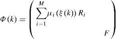
To estimate the unknown input, it is necessary that the matrix Φ(k) is of full column rank and its pseudo inverse Φ−(k) exists:
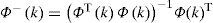
The unknown input can then be deduced:
We choose Φ(k) of full column rank, to reverse matrix (ΦT(k) Φ(k)).
Example 1:Reconstruction of state and estimation of unknown inputs by quadratic approach
Let us consider the following discrete multimodel:
In this example, the variable of decision ξ(k) is not measurable and depends on to the estimated vector of states x⌢k.
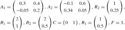
The numerical values of the matrices Ai, Bi, Ri, C and F are as follows:
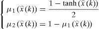
The activation functions have the following form:

The multiobserver able to estimate the multimodel (43) state is as follows:
The stabilization conditions given by proposition 1 prove the stability of the multiobserver (45), via the existence of quadratic function (16).
By applying the method of resolution presented in paragraph (3.2.1.1), we showed global convergence of the multiobserver (45).
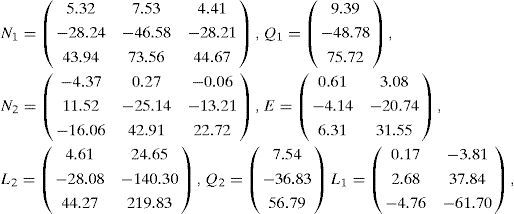
The resolution of the conditions of proposition 1 leads to the following result:
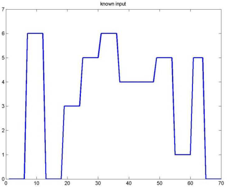
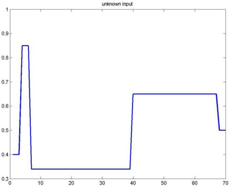
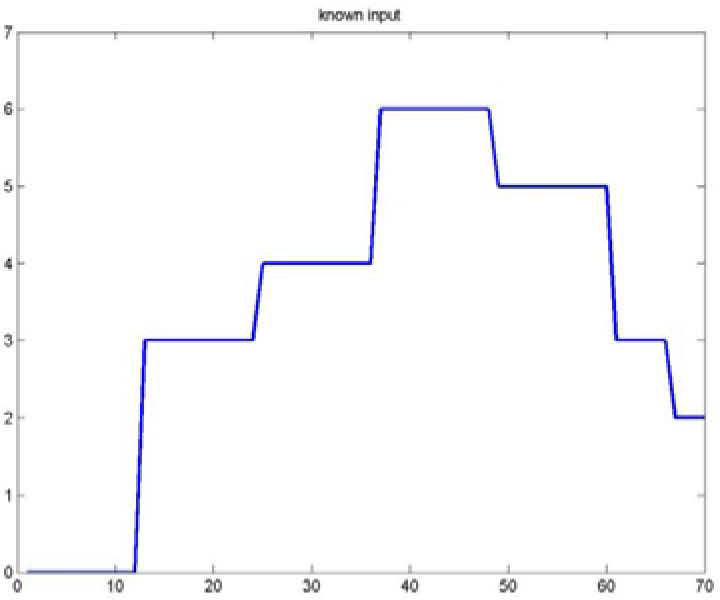
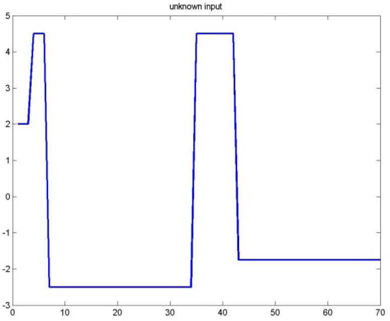
Figures 1 and 2 represents respectively the evolution of the inputs known u(k) and unknown u¯k.


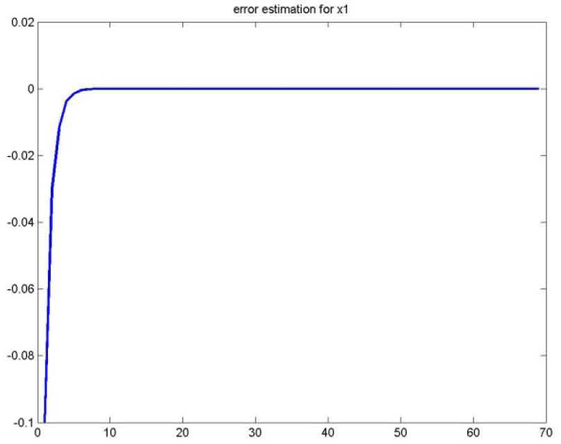
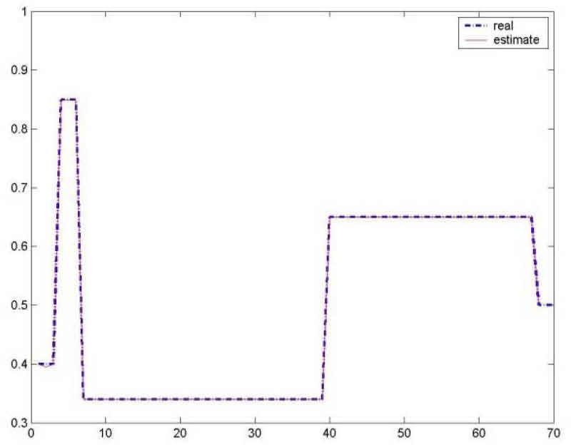
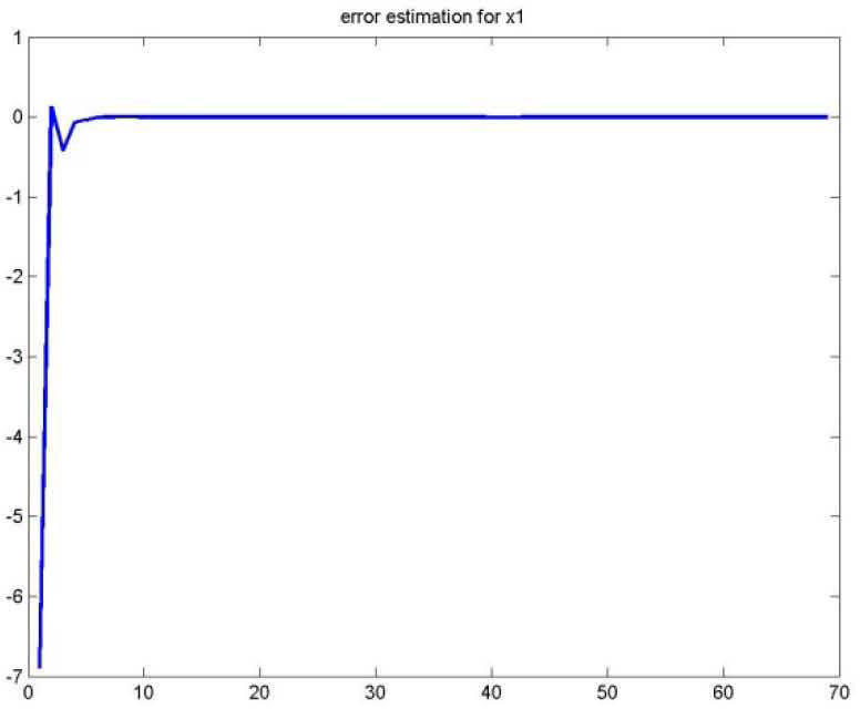
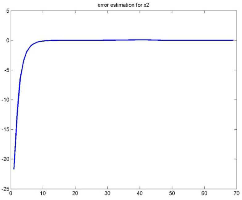
As for the figures 2, 3 and 5, they shows the state estimation errors xik−xˆik,i=1,2 as well as the unknown input u¯k of the multimodel and their estimation u¯⌢k.


It is noted that the estimation quality is satisfactory except in the vicinity of the origin time; that is due to the choice of initial values of the multiobserver (45).
Example 2: Conservatism of the quadratic approach
Let us consider the following discrete multimodel,

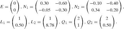
In this example, the variable of decision ξ(k) is not measurable but depending on the estimated vector of states x⌢k. The numerical values of the matrices Ai,Bi, Ri, C and F are as follows:
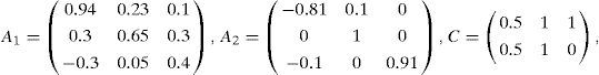
The activation functions have the following form:
The multiobserver able to estimate the multimodel (46) state is as follows:

The conditions of quadratic stabilization of proposition 1 fails to prove the stabilization of the multiobserver (48), which shows that no quadratic function having the form (16) can exist.
The quadratic approach becomes more and more conservative in the following cases:
- When the number of local models is very important, this is due to the difficulty to find one matrix P satisfying all (17) inequalities and equalities.
- When the multimodel have local saturated models (the eigen values of matrix Ai are closer to 1) like the local model number 2 (eigen values with A2 = {0.91, −0.81, 1 }).
Example 3: Reconstruction of state and estimation of unknown inputs by polyquadratic approachLet us consider the discrete multimodel of example 2; the conditions of stabilization of proposition 2 prove the stability of the multiobserver (48), which proves the existence of polyquadratic function of the form (29).
By applying the method described at paragraph (3.2.2.1), we ensure the global convergence of the multiobserver (48).
The resolution of the conditions of proposition 2 leads to the following result:
Figures 6 and 7 represents respectively the evolution of the inputs known u(k) and unknown u¯k.
.")
Evolution of Known input U (Example 3).

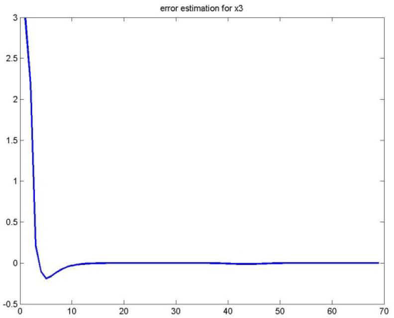
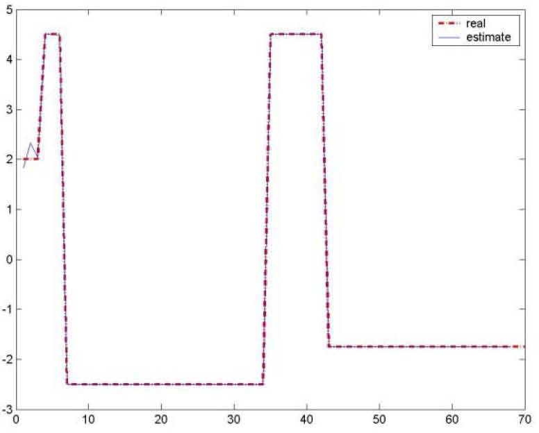
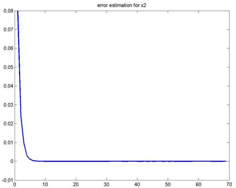
Figures 8, 9, 10 and 11 shows the state estimation errors xik−xˆik,i=1,2,3 as well as the unknown input u¯k of the multimodel and their estimation u¯⌢k.


It is noted that the estimation quality is satisfactory except in the vicinity of the time origin; that is due to the choice of the multiobserver (48) initial values.
Therefore, we observe good performances of the multiobserver estimation.
5Conclusions and prospectsIn this paper, we presented two stabilization approaches of a multiobserver with unknown inputs for a nonlinear system described by a discrete multimodel with non measurable decision variables. The first approach is based on the use of the Lyapunov quadratic functions, the conditions obtained from this approach for the convergence of the multi-observer are often easy to obtain but they appear pessimistic.
The second approach suggested for the stabilization of the observation error, is based on the use of the Lyapunov polyquadratic functions. The conditions obtained of the multiobserver convergence are given in the form of Bilinear Matrices Inequalities BMI that we can linearize by the technique of change of variables and easily solve them with the traditional numerical tools. This second approach appears less conservative than the first.
Two illustrative examples are considered to prove the efficiency and the effectiveness of the proposed approaches. The first example showed that the quadratic approach is interesting from point of view of the practical implementation for the supervision and the diagnosis of the industrial processes. The second example puts emphases on the important contribution of the polyquadratic approach compared to the quadratic approach for the states estimation and unknown inputs of a nonlinear system represented by a discrete multimodel.
Future work will relate to the poles placement of the multiobserver for unknown inputs, with the application to the diagnosis of the nonlinear systems.