


The generalized Shiryayev sequential probability ratio test (SSPRT) is applied to linear dynamic systems for single fault isolation and estimation. The algorithm turns out to be the multiple model (MM) algorithm considering all the possible model trajectories. In real application, this algorithm must be approximated due to its increasing computation complexity and the unknown parameters of the fault severeness. The Gaussian mixture reduction is employed to address the problem of computation complexity. The unknown parameters are estimated in real time by model augmentation based on maximum likelihood estimation (MLE) or expectation. Hence, the system state estimation, fault identification and estimation can be fulfilled simultaneously by a multiple model algorithm incorporating these two techniques. The performance of the proposed algorithm is demonstrated by Monte Carlo simulation. Although our algorithm is developed under the assumption of single fault, it can be generalized to deal with the case of (infrequent) sequential multiple faults. The case of simultaneous faults is more complicated and will be considered in future work.
Fault diagnosis has been extensively studied [1-10]. It can be addressed by hardware redundancy or analytical redundancy [4]. With the increasing computational power and decreasing cost of the digital signal processors and software, the method of analytical redundancy, which diagnoses the possible fault by comparing the signals from a real system with a mathematical model, is prevailing due to its low cost and high flexibility.
In this work, we study the fault diagnosis problem of a linear stochastic system subject to a single sensor/actuator fault. As pointed out in [3], the fault diagnosis problem consists of the following three sub-problems:
Fault detectionIs there a fault in the system? The answer is “yes”, “no” or “unknown”. It is actually a change detection problem with binary hypotheses. We want to detect the fault after its occurrence as quick as possible. For simple hypotheses with independent and identically distributed (i.i.d.) observations, optimal algorithms exist, e.g., cumulative sum (CUSUM) test [11], which (asymptotically) minimizes the worst-case expected detection delay under some false alarm restrictions [12, 13]. If the change time is assumed random and prior information is available, the Shiryayev sequential probability ratio test (SSPRT) [14] in Bayesian framework is optimal in terms of a Bayesian risk. Note that the fault source needs not to be identified (or isolated) in fault detection.
Fault isolation (or identification)Usually there are many components in modern systems and merely knowing there is a fault (by fault detection) in a system is far from enough for a quick and effective remedy. Hence, the goal of fault isolation is to identify the source of a fault as soon as possible. So, the answer to this problem is a fault type, e.g., which component in a system is faulty. This is a change detection problem with multiple alternative hypotheses. Each alternative hypothesis corresponds to a fault model (unlike fault detection, all the fault models are included in a single alterative hypothesis) and we need to isolate which hypothesis happens after a change. The fault isolation can be carried out subsequently after the fault detection (i.e., identifying the source after declaration of a fault) or individually (i.e., operates in a stand-along mode without the fault detection). Sequential algorithms for this problem were proposed in [6, 9] and it minimizes the worst-case expected isolation delay under the restriction of mean time before a false alarm/isolation. The generalized SSPRT (GSSPRT) in Bayesian framework was proposed [8] and it is optimal in terms of a Bayesian risk for fault isolation. To the authors’ best knowledge, joint optimal solution for fault detection and isolation is not known.
Fault estimationEstimate the severeness of a fault. For example, a sensor/actuator may fail completely (it does not work at all) or partially (has degenerated performance). This piece of information is useful for future decision and action. If a sensor/actuator fails completely, the system may have to be stopped until the faulty component is replaced or fixed. In another hand, if only minor partial fault occurs, the sensor/actuator may be kept in use, with some online compensation [3].
In this work, system state estimation, fault isolation and estimation are tackled simultaneously. We start from applying the GSSPRT to a linear dynamic system and the algorithm turns out to be a multiple model (MM) algorithm considering all possible model sequences [15]. Fault diagnosis by multiple model algorithms is gaining attentions. A bank of mathematical models is constructed to model the normal operation mode and the fault modes. Filters based on these models are running in parallel, and the system state estimation is obtained by the outputs from MM, and the fault isolation can be done by comparing the model probabilities with the pre-defined thresholds. So, the fault diagnosis and state estimation can be done simultaneously, and the performance of the state estimation is independent to that of fault diagnosis. The MM is attractive since it uses a bunch of models rather than a single model to represent the faulty behaviours of a system [10]. The autonomous multiple model (AMM) [15] algorithm was the first MM algorithm proposed for fault diagnosis [16-18]. However the underlying assumption of AMM about the model trajectory-the model in effect does not change over time-does not fit the change detection problem. Then, the interacting multiple model (IMM) [19] algorithm, which considers the interaction between models, was proposed [7, 10, 20, 21] and they outperform AMM in general. In [7], the IMM was directly applied to a fault isolation problem, but it was assumed that the fault models are exactly known. The hierarchical IMM [22] and IM3L [10] were proposed to address the fault isolation and estimation. However, they were tackled in a sequential manner, i.e., isolation-then-estimation. Without the information of the fault severeness, the isolation performance suffers. In this paper, we propose a multiple model algorithm that solves the fault isolation and estimation simultaneously.
In practical applications, each sensor/actuator fault can be total or partial. So, a parameter α ∈ [0, 1] is introduced for each sensor/actuator to indicate its fault severeness [7,10]. α = 0 means complete failure while 0 < α < 1 denotes a partial fault. If α is known after a fault occurrence, the hypothesis for each sensor/actuator fault becomes a simple hypothesis and the GSSPRT algorithm for this case is exactly the same as the MM algorithm considering all possible model sequences. Hence, the optimality of GSSPRT and the virtues of MM algorithms are all preserved. Further, the system state can be also estimated as a by-product. However, two difficulties impede its exact implementation in practice:
- a)
Its computational complexity is increasing due to the increasing number of model sequences.
- b)
α is unknown in general.
The first problem can be solved by pruning and merging the model sequences so that the total number of sequences is bounded. A bunch of algorithms were proposed for this purpose, e.g., B-best and GPBn, see [15] and the references therein. We propose to use the Gaussian mixture reduction [23, 24] to merge the “similar” model sequences, since it can be better justified than GPBn or IMM. Second, the unknown parameter α can be estimated online by model augmentation. We introduce one augmented model for each sensor/actuator with an (unknown) fault parameter α, which is updated at every step by maximum likelihood estimation (MLE) or expectation-the so-called maximum-likelihood model augmentation (MMA) [10, 20] or expected model augmentation (EMA) [15, 25], respectively. So, before declaration of a fault, the fault severeness has been estimated and updated in real time based on these augmented models. Further, these augmented models are expected to be “close” to the truth, and hence further benefit the overall performance of state estimation and fault isolation. As shown in the simulation, the EMA and MMA have their pros and cons to each other. The MMA has better adaptation of parameter change and hence has faster isolation and smaller miss detection rate, while the EMA performs better in terms of the parameter estimation and correct isolation rate.
Although our algorithm is developed based on the assumption of single fault, it can be extended to deal with infrequent sequential multiple faults easily provided the interval between two faults is long enough for isolating the first fault before the second fault. If a fault has been identified and its fault severeness estimated, then all the models can be revised to accommodate this fault and hence detection for further fault can be carried out. The case of simultaneous faults is more complicated and deserves further studies.
This paper is organized as follows. First, the problem of fault isolation and estimation for linear dynamic systems is formulated in Sec. 2. The algorithm based on GSSPRT is derived in Sec. 3. The multiple model methods based on the Gaussian mixture reduction and the model augmentation are presented in Sec. 4. Three illustrative examples are provided in Sec. 5, and our algorithms are compared with the IMM method. Conclusions are made in Sec. 6.
2Problem FormulationA linear stochastic system subject to a sensor/actuator fault can be formulated as the following first-order Markov jump-linear hybrid system:

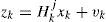
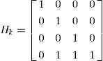
where xk and zk are the system state and the measurement at time k, respectively. Each column of Bk is an “actuator” while each row of Hk is a “sensor” in the system [7, 10, 21]. The superscript j denotes that the matrices dependent the model mj in effect. It is assumed that there are total M fault models {m1, m2,...,mM} and one normal model m0. The control input uk is assumed deterministic and known all the time. The process noise wk and measurement noise vk are Gaussian white noise with zero mean and covariances Qk and Rk, respectively. The model sequence {mk} is assumed to be a first-order Markov sequence with the transition probability
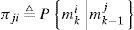
where mki denotes the event that mi is in effect at time k. The system usually starts with the normal model m00 and at each time k it has probability π0i >0 to transfer to mi (the i th fault model). Further, it is assumed that all fault models mi, i = 1,…,M, are absorbing state in the Markov chain, that is
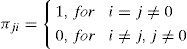
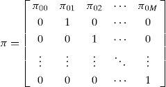
meaning that once a system gets into one of the fault models, it remains, since we only consider the case with single fault. The possibility that a system recovers automatically from a fault model is ignored since it rarely happens in practice. So, the transition probability matrix (TPM) is
The total and partial sensor/actuator faults are considered, and the fault models proposed in [7, 10] are adopted. Let αkj∈(0,1] denotes the severeness of the j th sensor/actuator’s fault at time k. The corresponding “actuator” in Bk or“sensor” in Hk is multiplied by αkj due to the fault. Clearly αkj=0 means that the sensor/actuator fails completely while 0<αkj<1 indicates a partial fault. In general, if a fault happens, αkj is unknown and time varying. The problem becomes much more difficult if αkj is fast changing. For simplicity, only a constant or a slowly drifting sequence is considered forαkj. If prior information is available, more sophisticated dynamic models for αkj are also optional.
Under these problem settings, we are trying to achieve the following three goals simultaneously based on sequentially available measurements Zk = {z1, z2,...,zk } :
- (a)
State estimation (xˆk|k) in real time;
- (b)
Fault identification (i.e., sensor/actuator jˆ);
- (c)
Fault severeness estimation αˆkj when a fault is identified.
Once a fault has been isolated and an estimate of the fault severeness is provided, additional actions based on these results can be taken to further inspect the decision and improve the estimation accuracy. This is problem dependent and there are many options, e.g., use a different model set specifically designed for the faulty sensor/actuator to achieve better state estimation and fault estimation. Also, the declared fault can be further tested against the normal model (or other fault models) to mitigate the possible false alarm (or false isolation) rate. We do not further examine these possibilities since they are beyond the scope of this paper.
3Generalized Shiryayev Sequential Probability Ratio TestFirst, we only consider the goal (b) and assume αkj is exactly known after a fault occurs. Then an optimal solution in Bayesian framework-generalized Shiryayev sequential probability ratio test (GSSPRT)-was proposed in [8] for this fault isolation problem. The optimality of GSSPRT was proved in terms of a Bayesian risk. Further, it minimizes the time of fault isolation given the costs of false alarm, false isolation and a measurement at each time k, see [8] for the proof and details.
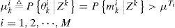
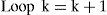
Assume the system starts with no fault. At each time k, the GSSPRT computes the posterior probability of the event θki ⃞ {Transition from m0 to mi occurs at or before time k}. and compares it with a threshold μTi,i=1,2,⃛,M. Once one of the thresholds is exceeded, the corresponding fault is declared. The optimal thresholds can be determined by the given costs [8]. Note that θk0 means the system remains in normal mode up to time k. The event θki is equivalent to the event mki since the fault model mi is an absorbing state in the Markov chain. The GSSPRT algorithm is summarized as follows:
Declare a sensor/actuator fault i if
Else, compute μk+1i,i=0,1,⃛,M,
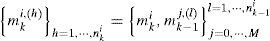
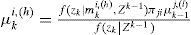
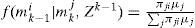
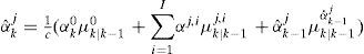
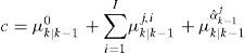
Note that in the algorithm there is no threshold set for m0 since declaration of the normal model is of no interest. The posterior probability μki is computed by
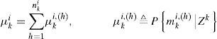
and mki,h denotes a model sequence which starts from time 0 and reaches model mi at time k, h is the index, and nki is the total number of such sequences. Since the system starts with no fault, mk0,h is the only valid sequence at time k = 0, and hence μ00,(1)=1. The probability μki,(h) can be computed recursively. Since
by Bayesian formula, we have
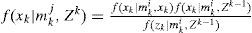
where the likelihood function f(zk|mki,(h),Zk−1) can be calculated based on the Kalman filter (KF) [26] under the linear Gaussian assumption. This can be done since the model trajectory has been specified by mki,(h)

where
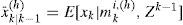
and Pˆk|k−1(h), is the error covariance matrix of x¯k|k−1(h) The model conditional density of the system state is
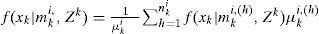
Clearly, f(xk|mki,Zk) is a Gaussian mixture density and the number of Gaussian components is increasing geometrically (i.e., (M + 1)k) with respect to k for a general TPM. However, due to the assumption that all the fault models are absorbing states (the special structure of Eq. (3)), it only increases linearly (i.e., MK+1) for our problem.
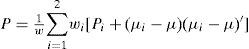
The estimate of xk and its mean square error (MSE) matrix can be obtained by:
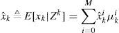
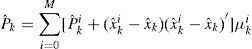
where
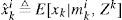
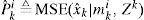
can be obtained from f(xk|mki,Zk) (Eq. (4)). xˆk is optimal in terms of the MSE.
The above procedure turns out to be the well-known cooperating multiple model (CMM) algorithm [15] considering all possible model trajectories. Before, the multiple model algorithm was developed for state estimation with model uncertainties. It is estimation oriented. Here, it is derived from a totally different angle by starting from GSSPRT for decision purpose. So, the goal (a) and (b) can be fulfilled simultaneously and optimally in terms of their criterions, respectively. Further, the state estimation is not affected by the performance of fault isolation.
Even a false alarm or false isolation occurs, the state estimation is still reliable, since the detection has no impact (or feedback) to the model-conditioned estimates and model probabilities, and hence does not affect the state estimation.
Besides the increasing computational complexity, the unknown fault parameters αkj in practical applications incur further difficulties to our algorithm. The hypothesis of a fault model becomes composite in this case, rendering it much more complicated. Further, it is usually very desirable that a good estimate of αkj can be provided at the time a fault is identified, meaning that αkj should be estimated online along with the fault identification process. The fault estimation can also provide useful information for fault isolation, and consequently benefits its performance.
4Multiple Model Algorithm Based on Gaussian Mixture Reduction and Model AugmentationFirst, we address the problem of computation complexity. As aforementioned, Eq. (4) is a Gaussian mixture density and its number of components is increasing rapidly. Each Gaussian component in f(xk|mki,Zk) corresponds to a model trajectory mki,(h). In real time implementation, the number of the components must be bounded.
In MM method, there are many algorithms proposed to reduce the number of model sequences [15]. They can be classified as: a} methods based on hard decision, such as the B-Best algorithm, which keeps the most likely one or a few model sequences and prunes the rest; b) methods based on soft decision, such as the GPBn algorithm, which merges those sequences with common model trajectories in last n steps (they may have different trajectories in older times). In general, the algorithms based on soft decision outperform those based on hard decision. However, for GPBn methods there is no solid ground to justify why sequences with common model steps should be merged. These common parts of model trajectories do not necessarily imply that the corresponding Gaussian components are “close” to each other. Consequently the merging may not lead to good estimation accuracy. We propose to use a more sophisticated scheme based on Gaussian mixture reduction, which involves both pruning and merging. The idea is simple and better justified, but requires more computation. However, in our problem, the number of model trajectories increases linearly instead of geometrically. The reduction process usually needs not to be performed frequently. Of course, this approach can be implemented for general MM algorithm, which may require the reduction for every step.
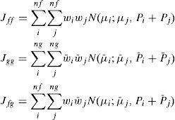
Once the number of components in f(xk|mki,Zk) exceeds a threshold, the extremely unlikely components can be pruned first. Then, the number of Gaussian components is further reduced to a pre-specified number by pairwise merging, with the grand mean and covariance maintained. This is the so-called Gaussian mixture reduction problem and was studied by [23, 24, 27-32]. The problem is to reduce the number of Gaussian components in a Gaussian mixture density by minimizing the “distance” (to be defined) between the original density and reduced density, subject to the constraint that the grand mean and covariance are unaltered. The optimal solution requires solving a high dimensional constrained nonlinear optimization problem that the weights, means and covariances are chosen such that the “distance” between the original mixture and the reduced mixture is minimized. This is still an open problem and optimal solution is computationally infeasible for most applications. However, a suboptimal and efficient solution is acceptable for our problem. As proposed in [23, 24, 30], a top-down reduction algorithm based on greedy method is employed. Two of the components are selected to merge by minimizing the “distance” between them at each iteration, until the number of components reduces to a pre-determined threshold. For two Gaussian components with weights wi, means µi and covariances Pi, they are merged by

so that the grand mean and covariance are preserved.
Further, there were many distances proposed for merging. They can be categorized to two classes: global distance and local distance. The global distance of two Gaussian components measures the difference between the original mixture density and the reduced mixture density (by merging these two elements), while the local distance only measures the difference between these two components. The global distance is preferred in general since it considers the overall performance. Kullback-Leibler (KL) divergence may be a good choice [30], but it cannot be evaluated analytically between two Gaussian mixtures, see [33] and reference therein for some numerical methods. An upper bound of KL divergence was proposed in [30] to serve as the distance, which is, however, a local distance. We adopt the distance proposed in [23, 24]-the integral squared difference (ISD). For two Gaussian mixture densities f(x) and g(x), the ISD is defined as
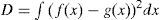
It is a global distance and can be evaluated analytically between any two Gaussian mixture
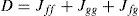
where
and {wi, µi, pi} and {w¯i,μ¯i,P¯i} are the weights, means and covariances, respectively, of the i th Gaussian components in f(x) and g(x). Efficient algorithms to compute the distance was proposed in [24]. Hence, the distance between two Gaussian components for merging is defined as
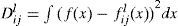
where f(x) is the original Gaussian mixture, fijl(x) is the mixture density after merging the i th and j th components in fl(x), which is the reduced Gaussian mixture at iteration l. For each iteration l, two components are selected to merge such that Dijl is minimized. The iteration stops when the number of the components reduces to the pre-specified number. Compare with the merging method in GPBn, the merging based on this Gaussian mixture reduction is better justified. Although the above reduction procedure does not reduce the Gaussian component optimally, it is based on a good guidance-only components that are “close” to each other are merged and hence the loss should be smaller than GPBn.
In MM algorithm, at time k − 1, assume the Gaussian mixture densities f(xk−1|mk−1j,Zk−1) and the model probabilities μk−1j for j = 0, 1, …, M are obtained. Then f(xk|mkj,Zk) can be updated recursively:
and the model probability μki
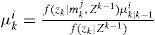
where


f(xk|mki,xk−1) and f(zk|mki,xk) are obtained from Eqs. (1) and (2), respectively. It can be seen from Eq. (5) that the number of the Gaussian components in f(xk|mkj,Zk) is increasing in each cycle. The Gaussian mixture reduction is implemented if necessary and f(xk|mkj,Zk) is replaced by the reduced density.
As mentioned before, due to the special structure of the TPM in our problem, the number of the Gaussian components increases linearly and hence the Gaussian reduction procedure needs not to be performed frequently.
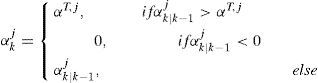
The second problem of applying the MM algorithm is the unknown parameter αkj for each sensor/actuator in the fault identification process. Before any fault occurrence, αkj=1 and it subjects to a possible sudden jump to a value that

Practically, only when αkj drops below a threshold αT,j < 1 it is considered as a fault:

Several methods may be applied to estimate αkj. It may be augmented into the system state. However, this requires a dynamic model for αkj, and the system becomes nonlinear (for sensor fault models) and subjects to a constraint. It can be also estimated by least squares method with fading memories [34, 35]. However, the abrupt change of αkj when a fault happens can incur difficulties for this algorithm. The method based on the maximum likelihood estimation (MLE) [10] is a good choice. For the j th sensor/actuator fault, a few models with different but fixed αkj (αkj=αj,i,i=1,2,⃛,I, where I is the number of fault models for the j th sensor/actuator) values and one augmented model with the parameter αkj estimated by the MLE in real time are included in the model set. The estimate αˆkj can be obtained by
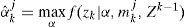
s. t. Eq. (7)
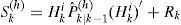
where, for simplicity, f(zk|α,mkj,Zk−1) can be approximated by a single Gaussian density, e.g., for a sensor fault, it yields
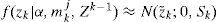
where

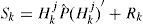

Since both z˜;k and Sk are functions of αkj, the MLE becomes a one-dimensional nonlinear inequality-constrained optimization problem which may be solved numerically. The MLE for an actuator fault can be obtained similarly, but the optimization procedure is simpler since it becomes a quadratic programming problem, which can be solved analytically by solving a linear equation. Then, the augmented models are updated by αkj in real time. This is the maximum likelihood model augmentation (MMA). It has a quick adaption in fault estimation when a fault occurs.
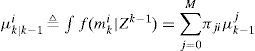
Another option is the expected model augmentation (EMA). It is similar to the MMA but the parameters αkj for the augmented models are estimated by weighted average of the models for the same sensor/actuator. That is, for a sensor/actuator fault j, the αˆkj for the augmented model is obtained by
is a normalizing constant, αk0≡1, μk|k−1αˆk−1j is the predicted probability of the augmented model, μk|k−1ij, are the predicted model probabilities of the models with fixed parameter αj,i. Note that this method circumvents the requirement of the constraint (Eq. (7)) since it is automatically guaranteed by the convex sum.
The augmented models in the model set serve two purposes: a) They are expected (hopefully) to be closer to the truth than the other models, and hence benefit the overall performance of the MM filter. b) The fault severeness can be obtained based on those augmented models, i.e., once a particular fault is declared, the corresponding αˆkj can be outputted as the fault estimate.
It is clear that the state estimation, fault isolation and estimation are solved simultaneously the a MM algorithm based on Gaussian mixture reduction and model augmentation. The results provide a basis for further diagnosis and actions. If, for example, a fault is declared but not sever or the faulty sensor/actuator is not critical, some online compensation can be applied to maintain the system in operation. Major action may have to be taken if a crucial or total failure occurs.
5Illustrative ExamplesWe provide three illustrative examples to demonstrate the applicability and performance of our algorithms by comparing with the results of IMM based on Monte Carlo (MC) simulation.
5.1Simulation ScenarioThe ground truth is adopted from [10, 21], i.e., a longitudinal vertical take-off and landing (VTOL) of an aircraft. The state is defined as
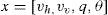
where the components are horizontal velocity (m/s), vertical velocity (m/s), pitch rate (rad/s) and pitch angle (rad), respectively. The target dynamic matrix and measurement matrix are obtained by discretization of the continuous system:

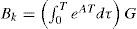
Where T = 0.1s is the sampling interval, and
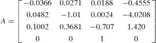
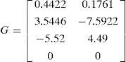
The control input is set to be uk = [0.2 0.05]′, the true initial state = [250 50 1 0.1]′, the covariances of the process noise Qk = 0.22I and the measurement noise Rk = diag[1, 1,0.1,0.1]. In this system, there are two actuators (A1 and A2) and four sensors (S1 – S4). The simulation lasts for 70 steps and the fault occurs at K = 10. The initial density of the state for the algorithms is chosen to be a Gaussian density N(x0,Pˆ0) with Pˆ0=diag[10,10,1,1].
5.2Performance MeasuresThe performances of our algorithms are evaluated by the following measures:
- 1.-
Correct identification (CI) rate: the rate that an algorithm correctly identifies a fault after it happens.
- 2.-
False identification (FI) rate: the rate that an algorithm incorrectly identifies a fault after it happens.
- 3.-
False alarm (Fa) rate: the rate that an algorithm declares a fault before any fault happens.
- 4.-
Miss detection (MD) rate: the rate that an algorithm fails to declare a fault within the total steps of each MC run.
- 5.-
Average delay (AD): the average delay (in terms of the number of sampling steps) for a correct isolation.
- 6.-
α⌣ the root mean square error (RMSE) of αˆ for a correct isolation.
All the performances are obtained by Monte Carlo simulation with 1000 runs. The thresholds for decision are determined by the results of simulation such that different methods have (almost) the same false alarm rate.
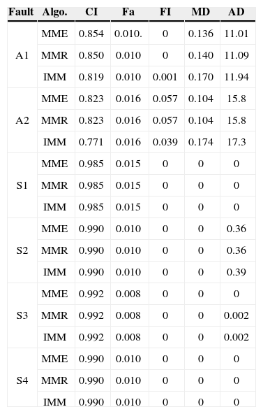
In this case, we consider the complete failure for each actuator/sensor. Hence, the fault severeness α = 0 is known. We compare the IMM, the exact MM (MME) method (i.e., considering all possible model trajectories) and the MM method based on the Gaussian mixture reduction (MMR). All the methods have the same model set of M + l models. It includes one normal model, and one fault model for each sensor/actuator.
There is no model-set mismatch between the algorithms and the ground truth. In MMR, the number of the Gaussian components for each model is reduced to 2 if it exceeds 10. This is a relative simple scenario since the fault parameter is known. The results are given in Table 1. It is clear that a sensor fault is much easier than an actuator fault to be identified.
Total fault, α = 0 and known.
| Fault | Algo. | CI | Fa | FI | MD | AD |
|---|---|---|---|---|---|---|
| A1 | MME | 0.854 | 0.010. | 0 | 0.136 | 11.01 |
| MMR | 0.850 | 0.010 | 0 | 0.140 | 11.09 | |
| IMM | 0.819 | 0.010 | 0.001 | 0.170 | 11.94 | |
| A2 | MME | 0.823 | 0.016 | 0.057 | 0.104 | 15.8 |
| MMR | 0.823 | 0.016 | 0.057 | 0.104 | 15.8 | |
| IMM | 0.771 | 0.016 | 0.039 | 0.174 | 17.3 | |
| S1 | MME | 0.985 | 0.015 | 0 | 0 | 0 |
| MMR | 0.985 | 0.015 | 0 | 0 | 0 | |
| IMM | 0.985 | 0.015 | 0 | 0 | 0 | |
| S2 | MME | 0.990 | 0.010 | 0 | 0 | 0.36 |
| MMR | 0.990 | 0.010 | 0 | 0 | 0.36 | |
| IMM | 0.990 | 0.010 | 0 | 0 | 0.39 | |
| S3 | MME | 0.992 | 0.008 | 0 | 0 | 0 |
| MMR | 0.992 | 0.008 | 0 | 0 | 0.002 | |
| IMM | 0.992 | 0.008 | 0 | 0 | 0.002 | |
| S4 | MME | 0.990 | 0.010 | 0 | 0 | 0 |
| MMR | 0.990 | 0.010 | 0 | 0 | 0 | |
| IMM | 0.990 | 0.010 | 0 | 0 | 0 |
A sensor fault can be detected (almost) immediately after the occurrence while it takes some time to detect an actuator fault. This makes sense because a sensor fault is directly revealed by the measurement while an actuator fault affects the measurement only through the system state.
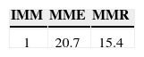
The performance differences among the three algorithms for a sensor fault are negligible, while MME and MMR evidently outperform the IMM algorithm for an actuator fault. But this superior performance is achieved at the cost of higher computational demands (given in Table 2). Comparing with MME, the performance loss of MMR is tiny.
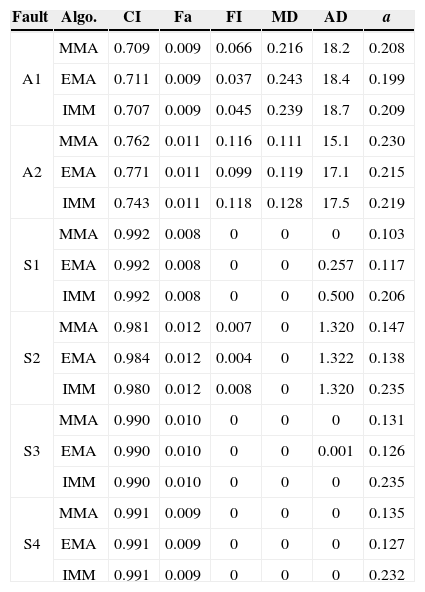
5.4Random ScenarioIn this case, for each MC run, the fault severeness αkj is sampled uniformly from the interval [0, αT,j] when a fault occurs and remains constant. The IMM, EMA and MMA (both based on Gaussian mixture reduction) are implemented and evaluated. The IMM contains 13 models: one normal model, two fault models for each sensor/actuator with a = 0 and 0.5, respectively. The EMA and MMA contain 19 models: all the models in IMM algorithm and one augmented model for each sensor/actuator. The results are given in Table 3. Similar to Case 1, a sensor fault is easier to be identified than an actuator fault, revealed by a shorter detection delay and better fault estimates. The performance differences among the three algorithms are insignificant for sensor faults. For actuator faults, MMA has a shorter detection delay and smaller miss detection rate, while EMA is better in terms of correct identification rate, false identification rate and estimation root mean square error. α⌣
Random fault, αT,j= 0.7.
| Fault | Algo. | CI | Fa | FI | MD | AD | a |
|---|---|---|---|---|---|---|---|
| A1 | MMA | 0.709 | 0.009 | 0.066 | 0.216 | 18.2 | 0.208 |
| EMA | 0.711 | 0.009 | 0.037 | 0.243 | 18.4 | 0.199 | |
| IMM | 0.707 | 0.009 | 0.045 | 0.239 | 18.7 | 0.209 | |
| A2 | MMA | 0.762 | 0.011 | 0.116 | 0.111 | 15.1 | 0.230 |
| EMA | 0.771 | 0.011 | 0.099 | 0.119 | 17.1 | 0.215 | |
| IMM | 0.743 | 0.011 | 0.118 | 0.128 | 17.5 | 0.219 | |
| S1 | MMA | 0.992 | 0.008 | 0 | 0 | 0 | 0.103 |
| EMA | 0.992 | 0.008 | 0 | 0 | 0.257 | 0.117 | |
| IMM | 0.992 | 0.008 | 0 | 0 | 0.500 | 0.206 | |
| S2 | MMA | 0.981 | 0.012 | 0.007 | 0 | 1.320 | 0.147 |
| EMA | 0.984 | 0.012 | 0.004 | 0 | 1.322 | 0.138 | |
| IMM | 0.980 | 0.012 | 0.008 | 0 | 1.320 | 0.235 | |
| S3 | MMA | 0.990 | 0.010 | 0 | 0 | 0 | 0.131 |
| EMA | 0.990 | 0.010 | 0 | 0 | 0.001 | 0.126 | |
| IMM | 0.990 | 0.010 | 0 | 0 | 0 | 0.235 | |
| S4 | MMA | 0.991 | 0.009 | 0 | 0 | 0 | 0.135 |
| EMA | 0.991 | 0.009 | 0 | 0 | 0 | 0.127 | |
| IMM | 0.991 | 0.009 | 0 | 0 | 0 | 0.232 |
This can be explained by the quick adaption of the change in α by MLE after the fault occurrence. It helps identifying the fault faster, but in general its estimation is less accurate than EMA and hence may increase the false identification rate. Overall, they outperform the IMM method.
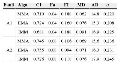
5.5Fault with Drifting ParameterIn this case, αkj is drifting after the fault. It is sampled uniformly from theinterval [0, αT,j] at the time of the fault occurrence and then follows a randomwalk (but bounded within [0, α T,j]), that is
where
and ℓk is uniformly distributed random samples (i.e., ℓk~U([−σ, σ] As mentioned before, a sensor fault is easier to be detected. It is identified (almost) immediately when it happens. So, in this case we only evaluate the performance for actuator faults. The results are given in Table 4. Compared with Case 2, the drifting αkj decreases the estimation accuracy and miss detection rate for both actuators, but increases the false identification rate significantly for actuator 1.
Fault with Drifting Parameter, where αT,j = 0.7 and σ = 0.02.
| Fault | Algo. | CI | Fa | FI | MD | AD | α⌣ |
|---|---|---|---|---|---|---|---|
| A1 | MMA | 0.710 | 0.04 | 0.188 | 0.062 | 14.8 | 0.220 |
| EMA | 0.724 | 0.04 | 0.160 | 0.076 | 15.3 | 0.208 | |
| IMM | 0.681 | 0.04 | 0.188 | 0.091 | 16.9 | 0.225 | |
| A2 | MMA | 0.745 | 0.08 | 0.106 | 0.069 | 15.6 | 0.236 |
| EMA | 0.755 | 0.08 | 0.094 | 0.071 | 16.3 | 0.231 | |
| IMM | 0.726 | 0.08 | 0.118 | 0.076 | 17.9 | 0.245 |
Applying the generalized SSPRT to a linear dynamic system for fault isolation and estimation leads to the multiple model algorithm. However, this algorithm must be approximated in real applications due to the increasing computational demands and the unknown fault parameters. The Gaussian mixture reduction (GMR) and model augmentations are proposed to address these two problems, respectively.
The GMR reduces the number of Gaussian components in a greedy manner by merging iteratively components that are “close” to each other. This merging algorithm is based on more solid ground than the conventional GPBn method for multiple model algorithms. Further, the fault parameters can be estimated based on the augmented models.
The model augmentations by expectation and MLE are good options. They have their pros and cons as indicated by the simulation results. The MLE provides a shorter fault isolation delay and an smaller miss detection while the EMA performs better in terms of the correct isolation rate and the estimation accuracy for the unknown parameter.
As mentioned before, the isolation and estimation of a fault provide a reference for further actions, and hence infrequent sequential faults can also be dealt with. The case of simultaneous faults is more complicated and is considered as future work.
Research was supported by the Fundamental Research Funds for the Central Universities (China), project No. 12QN41.