


In this paper, performance evaluation for various single model nonlinear filters and nonlinear filters with interacting multiple model (IMM) framework is carried out. A high gain (high bandwidth) filter is needed to response fast enough to the platform maneuvers while a low gain filter is necessary to reduce the estimation errors during the uniform motion periods. Based on a soft-switching framework, the IMM algorithm allows the possibility of using highly dynamic models just when required, diminishing unrealistic noise considerations in non-maneuvering situations. The IMM estimator obtains its estimate as a weighted sum of the individual estimates from a number of parallel filters matched to different motion modes of the platform. The use of an IMM allows exploiting the benefits of high dynamic models in the problem of vehicle navigation. Simulation and experimental results presented in this paper confirm the effectiveness of the method.
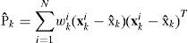
The synergy of Global Positioning System (GPS) [1,2] and inertial navigation system (INS) [1,3] has been widely explored due to their complementary operational characteristics. The GPS/INS integrated navigation system is typically carried out through the Kalman filter [1-2] to estimate the vehicle state variables and suppress the navigation measurement noise. In the Kalman filter or its nonlinear version, the extended Kalman filter (EKF), the state distribution is approximated by a Gaussian random variable (GRV), which is then propagated analytically through the first-order linearization of the nonlinear system.
Proposed by Julier, et al. [4], the unscented Kalman filter (UKF) is a nonlinear, distribution approximation method, which uses a finite number of carefully chosen sigma points to propagate the probability of state distribution through the nonlinear dynamics of system so as to completely capture the true mean and covariance of the GRV with a limited number sigma points by using the Unscented Transform (UT) [5-7]. The basic premise behind the UKF is it is easier to approximate a Gaussian distribution than it is to approximate an arbitrary nonlinear function. When the sample points are propagated through the true nonlinear system, the posterior mean and covariance can be captured accurately to the second order of Taylor series expansion for any nonlinear system. The particle filter (PF) [8-12] is a probability-based estimator. The Bayesian estimation is the foundation for particle filters. A large number of particles are required to obtain reasonable accuracy as the latest measurement is totally ignored. Henceforth, many variants of these filters are suggested by a number of researchers. To improve the estimate accuracy, the EKF or UKF can be used to generate the true mean and covariance of the proposal distribution.
The implementation of Kalman filter requires the a priori knowledge of both the process and measurement models. In various circumstances where there are uncertainties [13] in the system model and noise description, and the assumptions on the statistics of disturbances are violated due to the fact that in a number of practical situations, the availability of a precisely known model is unrealistic. The adaptive Kalman filters (AKF) [14-15] is used based on an on-line estimation of motion as well as the signal and noise statistics available data. Many efforts have been made to improve the estimation of the covariance matrices based on the innovation-based estimation approach, resulting in the innovation adaptive estimation (IAE).
The other approach is the multiple model adaptive estimate (MMAE). Proposed by Bar-Shalom and Blom, the interacting multiple model (IMM) algorithm [12,16-21] has the configuration that runs in parallel several model-matched state estimation filters, which exchange information (interact) at each sampling time. The IMM algorithm has been originally applied to target tracking [17-19], and recently extended to GPS navigation [20,21]. This algorithm carries out a soft-switching between the various modes by adjusting the probabilities of each mode, which are used as weightings in the combined global state estimate. The AKF approach is based on parametric adaptation, while the IMM approach is based on filter structural adaptation (model switching). In the IMM approach, multiple models are developed to describe various dynamic behaviors.
The remainder of this paper is organized as follows. In Section 2, the nonlinear filters are discussed. The IMM filter algorithm is introduced in Section 3. In Section 4, numerical simulation and experiment on navigation processing are carried out to evaluate the performance for various nonlinear filters in single-filter framework mode as well as in multiple-model framework. Conclusions are given in Section 5.
2The Nonlinear filtersGiven a single model equation in discrete time
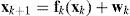
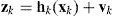
where the state vector xk ∈ ℜn, process noise vector wk ∈ ℜm, measurement vector zk ∈ ℜm, measurement noise vector vk ∈ ℜm, Qk is the process noise covariance matrix and Rk is the measurement noise covariance matrix.
2.1The extended Kalman filterThe vectors wk and vkin Eqs. (1) and (2) are zero mean Gaussian white sequences having zero cross-correlation with each other:
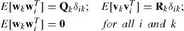
where E[·] represents expectation, and superscript “T” denotes matrix transpose. The symbol δik stands for the Kronecker delta function:
The discrete-time extended Kalman filter algorithm is summarized as follow:
- (1)
Initialize state vector and state covariance matrix: xˆ0|0 and P0|0 andP0|0
- (2)
Compute Kalman gain matrix:
- (3)
Update state vector:
- (4)
Update error covariancePk|k=[I –KkHk]Pk|k–1
- (5)
Predict new state vector and state covariance matrix


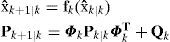
where the linear approximation equations for system and measurement matrices are obtained through the relations
2.2The unscented Kalman filter
Suppose the mean x¯ and covariance P of vector x are known, a set of deterministic vector called sigma points can then be found. The ensemble mean and covariance of the sigma points are equal to x¯ and P. The nonlinear function) y=f(x) is applied to each deterministic vector to obtain transformed vectors. The ensemble mean and covariance of the transformed vectors will give a good estimate of the true mean and covariance of y, which is the key to the unscented transformation.
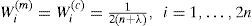
Consider an n dimensional random variable x, having the mean xˆ and covariance P, and suppose that it propagates through an arbitrary nonlinear function f. The unscented transform creates 2n+1 sigma vectors X (a capital letter) and weighted points W


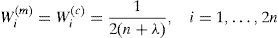
where ((n+λ)P)i is the ith row (or column) of the matrix square root. (n+λ)P can be obtained from the lower-triangular matrix of the Cholesky factorization; λ=α2 (n+k) – n is a scaling parameter; α determines the spread of the sigma points around x⌢ and is usually set as 1e – 4≤α≤1 ; k is a secondly scaling parameter usually set as 0; β is used to incorporate prior knowledge of the distribution of x¯;Wi(m) and Wi(c) are the weighs for the mean and covariance, respectively, associated with the ith point.

The sigma vectors are propagated through the nonlinear function to yield a set of transformed sigma points,

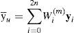
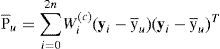
The mean and covariance of yi are approximated by a weighted average mean and covariance of the transformed sigma points as follows:
The implementation algorithm of UKF is summarized as follows:
- (1)
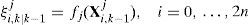
The transformed set is given by instantiating each point through the process model
ξi,k|k–1=fk–1(Xi,k–1),i=0,…, 2n
- (2)
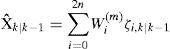
Predicted mean
- (3)
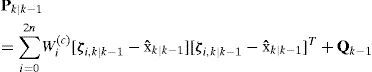
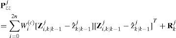
Predicted covariance
- (4)
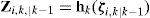
Instantiate each of the prediction points through observation model
- (5)
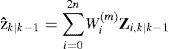
Predicted observation
- (6)
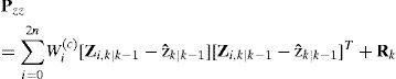
Innovation covariance
- (7)
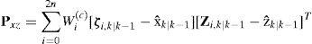
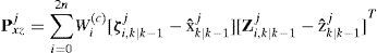
Cross covariance
- (8)
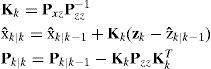
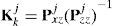
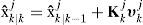
Performing update
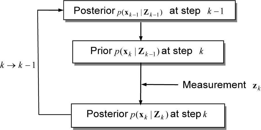
Although the EKF and UKF can deal well with some nonlinear filtering problems, however, they always approximate p(xk | zk) to be Gaussian, where p(xk | zk)=pdf of xk conditioned on measurements z1, z2, …, zk. The particle filter is a probability-based estimator. If the true density is non-Gaussian, particle filters may lead to better performances in comparison to that of EKF or UKF. Figure 1 shows the recursive Bayesian state estimation, which is based on the Bayes’ rule

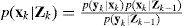
In order to compute p(xk | zk), the equation p(xk | zk-1), needs to be found from the Chapman-Kolmogorov equation and the marginal density function:

The pdf p(zk | zk-1) can be obtained to be

The basic PFs combine two principles namely the Monte Carlo (MC) principle and the Importance Sampling (IS) method where the transition prior density p(xk | xk-1) is taken as the importance distribution:

The weights of these particles are evaluated according to:
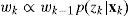
and

where q(xk | xk−1,zk) is the importance density function, wk–1 are the importance weights of the previous epoch particles and wk are the importance weights of the current epoch.
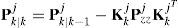
2.4The extended Kalman particle filter and unscented particle filterThe extended Kalman particle filtering (EKPF) is formed when the EKF is used for the importance proposal generation [9]; the unscented particle filter (UPF) is formed when the UKF is used for the importance proposal generation [8]. In a local linearization technique, such as the EKPF and UPF, each particle is drawn from the local Gaussianapproximation of the optimal importance distribution p(xk | xk−1,zk) that is conditioned on that is conditioned on the current state and the latest measurement

where qN denotes the Gaussian approximation of importance density and is obtained from EKF/UKF.
An improvement in the choice of proposal distribution over the simple transition prior can be accomplished by moving particles towards the regions of high likelihood, based on the most recent measurement. An effective approach to accomplish this is to use an EKF or UKF generated Gaussian approximation optimal proposal [4,6]

where xki and Pki are the mean and covariance of the ith particle generated by the EKF/UKF, respectively. This is accomplished by using a separated EKF or UKF to generate and propagate a Gaussian proposal distribution for each particle.
One cycle of the EKPF/UPF (i.e., the PF that uses EKF/UKF as proposal distribution) algorithm can be summarized as follows.
(1) Initialization. Assume {x0i}i=1N be a set of particles sampled from the prior x0i~p(x0) at k=0 and set
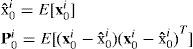

where i=1…N
(2) Importance sampling
(i) Update each particle with the EKF/UKF to obtain mean x¯ki and covariance Pki.
(ii) Sample the particles from

where xˆkiPki are the estimation of mean and covariance of EKF/UKF, i=1,…,N.
(iii)The recursive estimate for the importance weights can be written as follows
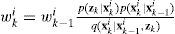
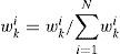
where N is the number of samples. Normalized the importance weights by
(3)Selection or re-sampling. Compute the effective weights according to
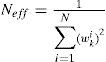
If Neff<N, resample particles {xki}i=1N and assign equal weights to them wki=1/N.
(4)Output
3The interacting multiple model (IMM) filter framework
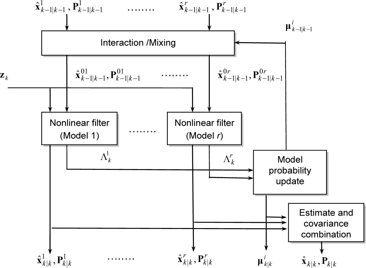
The IMM approach carries out a ‘soft switching’ among various models by the model probability. The algorithm of IMM-nonlinear filters is introduced to deal with the noise uncertainty and system nonlinearity simultaneously. Figure 2 describes the structure of the IMM estimator for the case of r models.
.")
Let a general system for multiple models in discrete time be described by


where fk(·) and hk(·) are the parameterized state transition and measurement functions, xk and fk are the dynamical state and measurement of the system in model Mk, and the system itself is a Markov chain, wk, vk are the process noise and measurement noise with means w¯k,v¯k and covariances Qk and Rk, respectively.
3.1IMM-EKFAn IMM cycle consists of four major stages. The IMM-EKF algorithm is summarized as follows.
(1) Model interaction/mixing. For given states xk−1j=xk−1|k−1j with corresponding covariances Pk−1j=Pk−1/k−1j and mixing probabilities μk−1|k−1i|j for every model, the initial condition for the model j is
The covariance corresponding to the above is:

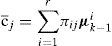
Calculating the mixing probabilities with mode switching probability matrix πij and the Gaussian mixing probabilities are computed via the equations:
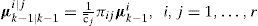
where c¯j is a normalization factor is
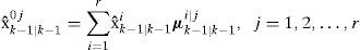
where xˆk−1|k−10j and Pˆk−1|k−10j are the mixed initial condition for mode-matched filter j at time k – 1. Note that, in this context, i and j denote the corresponding model index respectively; n is the total number of sampling particles.
(2) Filtering. The state estimate equation and covariance equation are used as input to the filter matched to Mkj, which uses zk to yield xˆk|kj and Pk|kj. The likelihood function corresponding to the r filters
are computed using the mixed initial condition as
(3) Model probability update. Model probability is updated according to the model likelihood and model transition probability governed by the finitestate Markov chain:

where

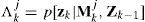
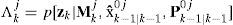
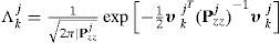
and Λkj is a likelihood function given by
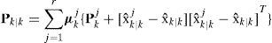
(4) Combination of state estimation and covariance combination. Combination of the modelconditioned estimates and covariances is done according to the mixture equations
3.2IMM-UKF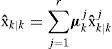
One cycle of the IMM-UKF is similar to that of the IMM-EKF except that the EKF used in the IMMEKF is replaced by the UKF, as follows.
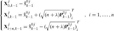
(1) Step 1 in UKF. The unscented transform creates 2n+1 sigma vectors X (a capital letter) and weighted points W. For state estimation at instant k – 1, sigma points are generated according to


(2) Step 2 in UKF. Time update (prediction steps)
(3) Step 3 in UKF. Measurement update (correction steps)
where υkj=Zk−zˆk|k−1j.
The samples are propagated through true nonlinear equations; the linearization is unnecessary, i.e., calculation of Jacobian is not required.
3.3IMM-EPFThe extended particle filter (EPF) with IMM framework yields the IMM-EPF. Integrating a bank of extended Kalman particle filters with the IMM method, an IMM-EKPF is obtained [12]; integrating a bank of unscented particle filters with the IMM method, an IMM-UPF is obtained. One cycle of the IMM-EPF (IMM-EKPF or IMM-UPF) is similar to that of the IMM-EKF or IMM-UKF except that the filters are replaced by the extended particle filters (i.e., EKPF or UPF).
4Results and discussion for GPS/INS integrationThe differential equations describing the two-dimensional inertial navigation state, where two accelerometers and one gyroscope are involved, are:
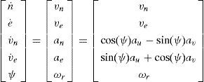
where [au, av] are the measured accelerations in the body frame, ωr is the measured yaw rate in the body frame. The error model for INS is constructed by the navigation states augmented by the accelerometer biases and gyroscope drift:
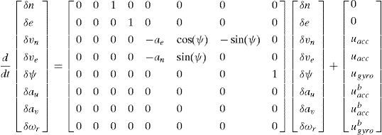
which were utilized in the integration Kalman filter as the inertial error model. In Eq. (57), δn and δe represent the east, and north position errors; δvn and δve represent the east, and north velocity represent the east, and north velocity δψ represents yaw angle; δau, δav, and δωr represent the accelerometer biases and gyroscope drift, respectively. The measurement model is
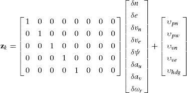
The GPS-derived yaw angle measurement can be obtained through

Simulation and experimental tests have been carried out to evaluate the navigation performance for the proposed approach in comparison with the conventional approaches.
A. Simulation example. The navigation integration software was developed by the authors using the Matlab® software. The commercial software Satellite Navigation (SATNAV) toolbox [22] by GPSoft LLC was employed for generating the satellite positions and pseudoranges.
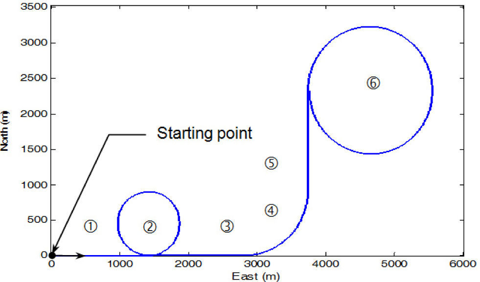
Figure 3 shows the schematic illustration of simulated trajectory. The trajectory can be divided mainly into six time intervals (or segments) according the dynamic characteristics, as indicated in the figure. The vehicle was simulated to conduct constant-velocity straight-line during the three time intervals, 0-45, 135-180 and 225-270s, all at a constant speed of 10π m/s. Furthermore, it conducted circular motion with radius 450 meters during 45-135s (counterclockwise); with radius 900 meters during 180-225s (counterclockwise) and 270-450s (clockwise) where high dynamic and medium maneuverings are involved.

Assume that the differential GPS (DGPS) mode is used and only multipath and receiver thermal noise are considered. The measurement noise variances rρi are assumed a priori known, which is set as 9m2. Let each of the white-noise spectral amplitudes that drive the random walk position states be sec Sp=0.003 (m / sec2)/rad/sec. Also, let the clock model spectral amplitudes be Sf=0.4(10-18)sec and Sg=1.58(10-18)sec-1. The measurement noise covariance matrix is given by Rk=15×Im×m.
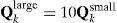
100 particles were used whenever the particle filter (for both EKPF and UPF) is used. For the two models of the IMM algorithms, two process noise covariance matrices are used: Qksmall=(1e−3)×I8×8, Qklarge=5Qksmall. The mode transition matrix is given by
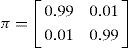
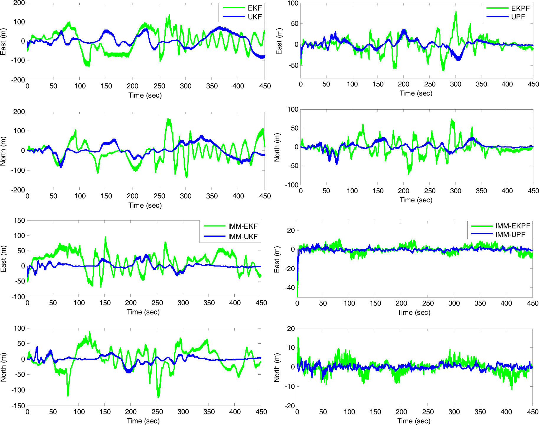
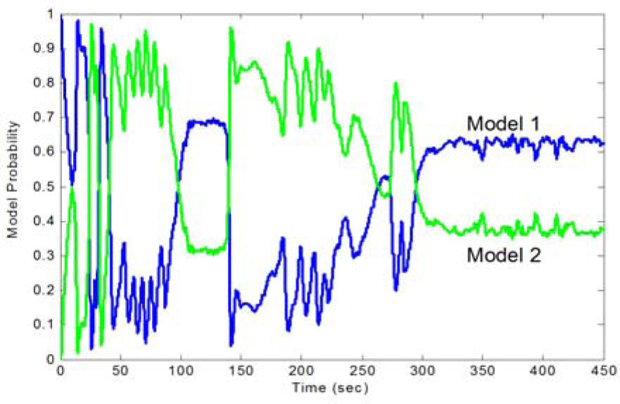
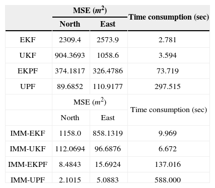
The UKF parameters are: α=1 κ=0, β=2. Figure 4 gives the results for the simulated case for various nonlinear filters, in single-model and IMM frameworks. The corresponding model probability is shown in Figure 5. Table 1 provides the comparison of position errors using nonlinear filters and IMM nonlinear filters for the simulation case.


Comparison of position errors using nonlinear filters and IMM nonlinear filters – simulation results.
| MSE (m2) | Time consumption (sec) | ||
|---|---|---|---|
| North | East | ||
| EKF | 2309.4 | 2573.9 | 2.781 |
| UKF | 904.3693 | 1058.6 | 3.594 |
| EKPF | 374.1817 | 326.4786 | 73.719 |
| UPF | 89.6852 | 110.9177 | 297.515 |
| MSE (m2) | Time consumption (sec) | ||
| North | East | ||
| IMM-EKF | 1158.0 | 858.1319 | 9.969 |
| IMM-UKF | 112.0694 | 96.6876 | 6.672 |
| IMM-EKPF | 8.4843 | 15.6924 | 137.016 |
| IMM-UPF | 2.1015 | 5.0883 | 588.000 |
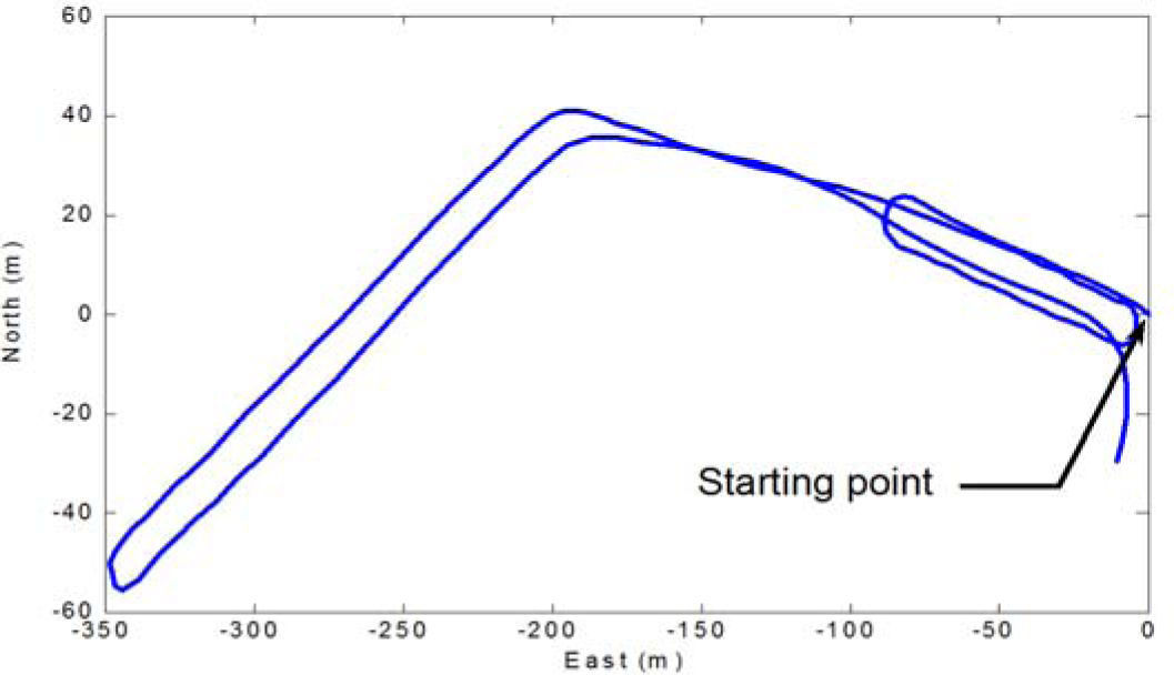
B. Road test. The road test was conducted in Hsinchu, Taiwan. The test drive results were obtained by post processing of logged sensor data using the Matlab® software. The GPS data was used as reference trajectory for comparative study on navigation performance for various dynamic environments using various nonlinear with/without IMM framework. The Micro-ElectroMechanical-Systems (MEMS) inertial sensors used were the BOSCH SMB380 Triaxial acceleration sensors and the XV–8000CB Ultra Miniature Size Vibration Gyro Sensors. The GPS data was collected at 1 Hz and the IMU has a data rate of 10 Hz. The driving speed is around 16~25km/hr for most of the time. Two process noise covariance matrices are used:
where
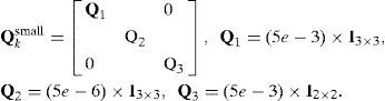
In this experiment, Figure 6 shows the trajectory for the road test.

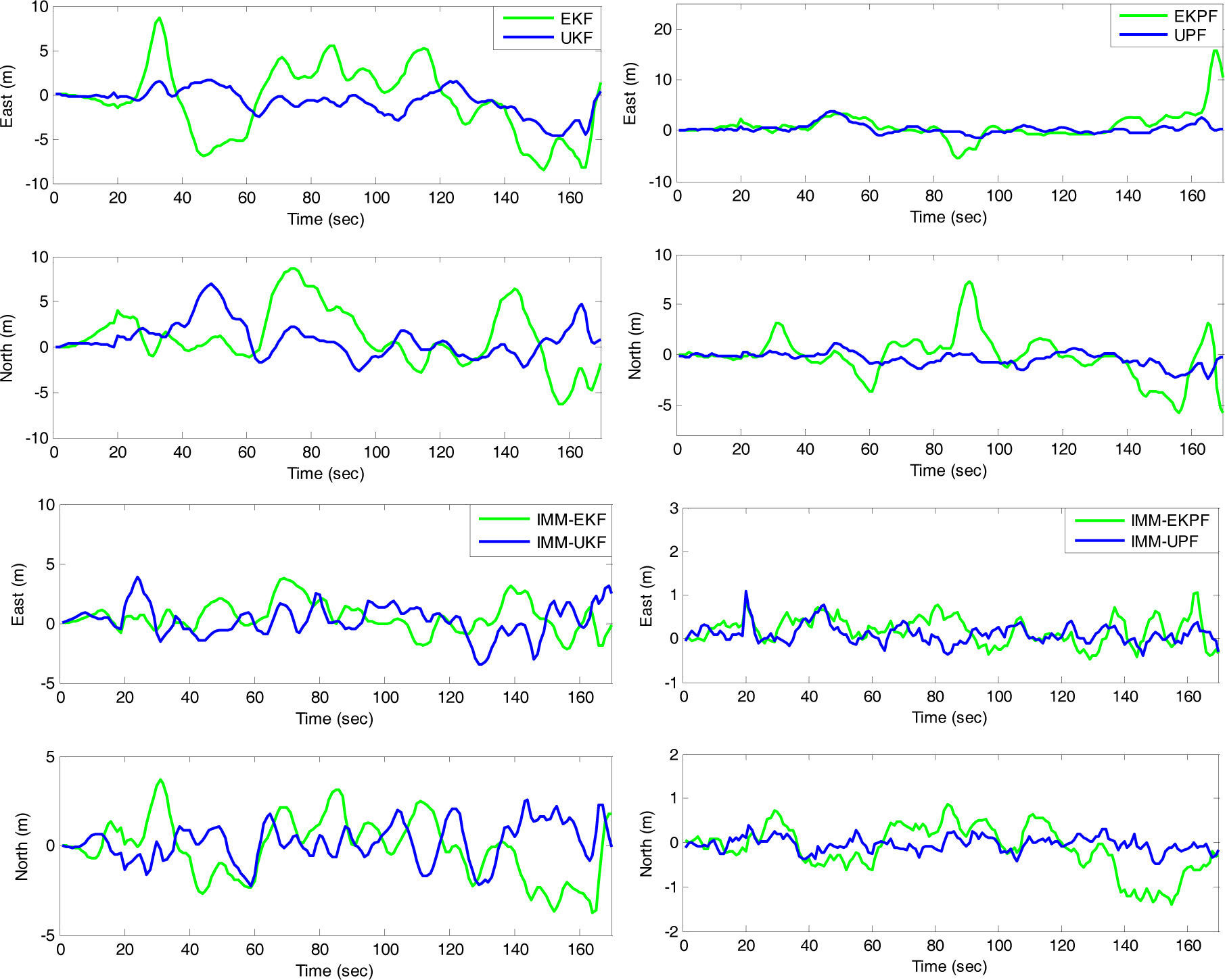
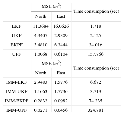
The results are illustrated in Figure 7. Table 2 shows comparison of position errors and computation time using various nonlinear filters and IMM nonlinear filters. When trials with sharp turns and abrupt maneuvers are performed, the performance enhancement becomes remarkable. It can also be seen that the computational load for the particle filter has been rapidly increased. The number of particles used in the test is 100. The number of sigma points in the UKF is 2n+1, which is 17 in this paper.

Comparison of position errors using nonlinear filters and IMM nonlinear filters – experiment results.
| MSE (m2) | Time consumption (sec) | ||
| North | East | ||
| EKF | 11.3684 | 16.0626 | 1.718 |
| UKF | 4.3407 | 2.9309 | 2.125 |
| EKPF | 3.4810 | 6.3444 | 34.016 |
| UPF | 1.0068 | 0.6104 | 157.766 |
| MSE (m2) | Time consumption (sec) | ||
| North | East | ||
| IMM-EKF | 2.9483 | 1.5776 | 6.672 |
| IMM-UKF | 1.1663 | 1.7736 | 3.719 |
| IMM-EKPF | 0.2832 | 0.0982 | 74.235 |
| IMM-UPF | 0.0271 | 0.0456 | 324.781 |
This paper has presented comparative study on navigation performance for various nonlinear filters, including EKF UKF EKPF UPF. Furthermore, the nonlinear filters have been incorporated into the interacting multiple model framework, resulting in the IMM-EKF IMM-UKF IMM-EKPF IMM-UPF algorithms. The problem of filter parametric adaptation can be regard as the generalization of structural adaptation. To solve the possible degradation problem caused by noise uncertainty and modeling error, the IMM algorithm can be employed for dynamically adjusting the process noise, and accordingly enhancing the estimation accuracy. However, selection of the nonlinear filters in the IMM framework leads to different levels of computational burden. The IMMPF requires significantly large computational time as compared to the other two algorithms. Trade-off needs to be made when selecting a suitable algorithm for a specific purpose.
Funding for this work was provided by the National Science Council of the Republic of China under grant numbers NSC 97-2221-E-019-012 and NSC 98-2221-E-019-021-MY3.