


This paper presents an evolutionary algorithm based technique to solve multi-objective feature subset selection problem. The data used for classification contains large number of features called attributes. Some of these attributes are not relevant and needs to be eliminated. In classification procedure, each feature has an effect on the accuracy, cost and learning time of the classifier. So, there is a strong requirement to select a subset of the features before building the classifier. This proposed technique treats feature subset selection as multi-objective optimization problem. This research uses one of the latest multi-objective genetic algorithms (NSGA - II). The fitness value of a particular feature subset is measured by using ID3. The testing accuracy acquired is then assigned to the fitness value. This technique is tested on several datasets taken from the UCI machine repository. The experiments demonstrate the feasibility of using NSGA-II for feature subset selection.
The feature subset selection has become a challenging research area during the past decades, as data sets used for classification purposes in data mining are becoming huge horizontally as well as vertically. Most of the data sets used for classification contain large a number of features (attributes) that are not all relevant. But all these features are used as input to the classification algorithm due to lack of sufficient domain knowledge. Each feature used as a part of the input causes increase in the cost and running time of the classification algorithm and may reduce its generalization ability and accuracy. So there is a huge need for a technique that can find smallest possible feature subset that has high classification accuracy. The multi-objective problems contain more than one objective to be optimized at one time. Most of the real world problems are multi-objective in nature. The feature subset selection problem may also be considered as one of them. The multiple objectives to be optimized simultaneously are the accuracies of the different classes in a data set. Efforts to increase accuracy of one class may reduce the accuracy of another class. This research treats feature subset selection problem as multi-objective problem and uses a multi-objective genetic algorithm to solve it. Multi-class problem has been converted into two-class problem because this research wants to increase the accuracy of each class as a separate objective (equally important). The fitness of each class is evaluated separately, after converting it into two class problem.
There are basically two approaches to solve multi-objective optimization problem. First is ideal multi-objective optimization procedure [14], that finds multiple trade-off optimal solutions and then chooses one of the obtained solutions using higher level information. The second approach is preference-based-multi-objective optimization procedure [14], that first chooses a preference vector and this vector is then used to construct the composite function, which is then optimized to find a single trade-off optimal solution by a single objective optimization algorithm. The most striking difference in single objective and multi-objective optimization is that in multi-objective optimization the objective functions constitutes an additional multi-dimensional space in addition to the usual decision variable space in the case of single objective function. This additional space is called the objective space [14]. When there are multiple objectives to be optimized simultaneously most researchers make use of the concept of non-dominated or Pareto optimal set of solutions. To understand the concept of non-domination, it is better to understand the concept of domination first. A solution x is said to dominate the other solution y if the solution x is no worse than y in all objectives and the solution x is strictly better than y in at least one objective [14]. There are other approaches using neural network [20], evolutionary multi agent system [21], evolutionary algorithm [22, 25], a hybrid of evolutionary algorithm and neural network [23], approaches using genetic algorithm with particle swarm optimization [24], hybrid evolutionary algorithm [26], and using multi-objective approaches for heuristic optimization [27] for optimization and classification problems. The evolutionary based technique has been used as it works well for the problems with large dimensions, it is known to be a robust technique and it works well with all types of problems because it does not make any assumptions about underlying fitness landscape.
The main features of the proposed method are:
- •
This research treats feature subset selection as a multi-objective optimization problem.
- •
The accuracy of each class is considered as a separate objective to be optimized
- •
This technique makes feature subset selection non-rigid.
- •
It gives the choice to the user to choose one of the feature subsets in the Pareto-front according to his needs.
- •
The selected feature subset by the proposed algorithm gives better accuracy and helps to produce less complex classifier.
Feature subset selection is the problem of selecting a subset of features from a larger set of features based on some optimization criteria. Some of the features in the larger set may be irrelevant or mutually redundant. Each feature has an associated measurement cost and risk. So, an irrelevant or redundant feature can increase the cost and risk unnecessarily. The choice of features that represent any data affects several aspects including [15]: Accuracy: The features that describing the data must capture the information necessary for the classification. Hence, regardless of the learning algorithm, the amount of information given by the features limits the accuracy of the classification function learned. Required learning time: The features describing the data implicitly determine the search space that the learned algorithm must explore. An abundance of irrelevant features can unnecessarily increase the size of the search space and hence the time needed for learning a sufficiently accurate classification function. Cost: There is a cost associated with each feature of the data. In medical diagnosis, for example, the data consists of various diagnostic tests. These tests have various costs and risks; for instance, an invasive exploratory surgery can be much more expensive and risky than, say, a blood test. Taking into consideration the above mentioned aspects that are affected by the selection of feature subset, the main objectives for feature subset selection are:
- •
Improvement in accuracy of the classifier,
- •
Prediction through a classifier quickly,
- •
Reduction in the cost
The performance of the classifier depends on many parameters, such as size of training set, number of features and the classifier complexity. If the training set remains the same and number of features increase, the performance of classifier is degraded [9]. As a result, one should minimize the number of irrelevant features which is also known as dimensionality reduction.
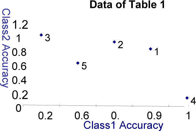
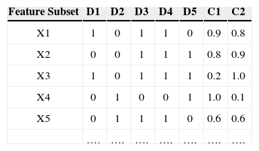
3Multi-objective Evolutionary AlgorithmIn feature subset selection problem, multi-objectives comes in naturally. Table 1 shows an example of different feature subsets (solutions) where Di are the features marked as 1 for being present or 0 for being absent. This data has two classes C1 and C2. The accuracies of the feature subset for both the classes are shown in the last two columns.
If a feature subset X1 is selected, it gives 90% accuracy for a particular class say C1 but does not work equally good for class C2(e.g. 80% accuracy). Similarly there is another feature subset called X2. This subset of features gives 90% accuracy for class C2 but does not work equally well for class C1. These two feature subsets are considered to be non-dominated to each other as X1 is better for C1 while X2 is better for C2. But if another feature subset X3 provides 20% accuracy to class C1 and 10% accuracy to class C2, this feature subset is inferior to the last two feature subset (solutions). So the accuracies may be considered as multiple objectives for multiple classes hence a multi-objective technique may be used to find better results.
The accuracies shown in Table 1 are plotted on the graph shown in Figure 1. It can be clearly seen that feature subset X1 and X2 must be preferred as they have balanced and better accuracies. So considering different class's accuracies as different objectives to meet makes the feature subset selection non-rigid.

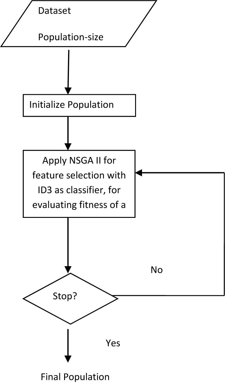
If the user decides that the accuracy of one class is more important than the accuracy of another class then he will have the option to select a feature subset (from the feature subsets on the non-dominated front) which fulfills his needs. If, for a problem, all the class accuracies are important then the user can select a subset which gives high, but balanced accuracies. It may also transpire, for a given dataset, that one of the subsets may dominate all other subsets. This research uses NSGA II due to improved complexity and the use non domination. The main algorithm is presented with the help of a flow chart shown in Figure 2.

The selection of non-dominated points in search space takes into consideration the accuracies of all the classes. The feature subset selection is carried out through NSGA II. The fitness function uses ID3 classifier for calculating the fitness of each candidate feature subset. ID3 algorithm has been used because it requires smallest amount of pre-processing, it is a robust decision tree algorithm and works well for large datasets.
3.1Input ParametersThe parameters used as input to this algorithm are
- •
Population size
- •
Number of generations
- •
Data set (number of attributes, number of classes)
Dataset must be of nominal type as ID3 works for nominal data only. The number of attributes is the total number of features a dataset contains. The number of classes is the number of objectives to be optimized.
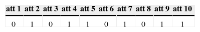
3.2Population InitializingThe number of chromosomes initialized is equal to the population size given by the user. Each chromosome is a binary string of size equal to total number of features in the data set. The Table 2 represents an example of a single chromosome which is a string of binary numbers (0 or 1) where 0 represents the absence of a feature and 1 represents the presence of a feature. The assumption in the example is that there are 10 attributes in total in this data set. This chromosome represents the presence of attributes 2, 4, 5, 7, 9 and 10. These binary strings are initialized randomly in the beginning.
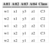
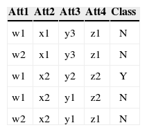
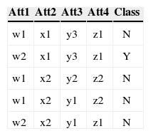
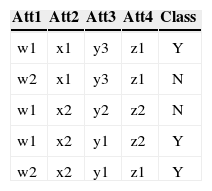
3.3Conversion of Multiple to Two Class ProblemAs mentioned before each class's accuracy is an objective so there is a need of converting a multiple class problem into two class problem for each class in the dataset. This conversion is necessary because the fitness of each class needs to be evaluated separately. For the conversion the concerned class is labeled as Y while all the other classes are labeled N. For example consider a data with four attributes, three classes (C1, C2 and C3), and five instances as shown in Table 3 (a).
As this data set has three classes so this data has been converted into three two class problems. The Table 3 (a) shows the data as multi-class data. The Table 3 (b) shows the two class problem for C1 (class 1). The instances that have C1 as their class are replaced by Y (true) as their new class, while class of rest of the four instances are replaced by N (false). Comparing Table 3 (a) and 3 (b) show that the class of third instance has been replaced by Y while the rest of instances now have class N. The conversion for C2 (class 2) and C3 (class 3) is shown in Table 3 (c) and (d) respectively.
Before any chromosome is evaluated, the data is trimmed according to the feature subset represented by the chromosome. The data is trimmed by deleting the columns of those attributes that are not present in that particular feature subset. After that this trimmed data is evaluated.
3.5Evaluation FunctionEvaluation function calculates the fitness of each feature subset (solution) in the current generation. The fitness for each chromosome is evaluated by first applying ID3 algorithm on training data for each converted class (see section 3.3).The decision tree is the output of ID3 algorithm. The testing data is tested on the decision tree and is then used to calculate the accuracy of the chromosome. The percentage of the instances of the testing data correctly classified by the decision tree is the accuracy of the chromosome. For example, testing data has 20 instances and 15 out of them are correctly classified. Then the accuracy of the chromosome will be 75% which is basically the fitness of the chromosome. This process is repeated five times for each chromosome with different training and testing data as five-fold cross validation is used by this technique to authenticate the results properly (Section 4.5). This evaluation function creates five trees for each chromosome in a population and for each class. The accuracies for all these five trees are averaged to get the final accuracy for each class for each chromosome.
This research treats the feature subset selection as multi-objective problem where these multiple objectives are the highest accuracy for each class separately. The fitness value for each class is considered as a fitness value of single objective in a multi-objective space. The selection of a particular chromosome depends on the fitness values of all the class and the distance of that chromosome from other chromosomes.
3.6Applying NSGA-IIThe population is initialized and is then sorted based on non-domination into each front. The sorting is done after evaluating each candidate subset. As stated before according to the candidate feature subset, the data is trimmed and is then passed on to the evaluation module. Each candidate feature subset in each front is assigned a rank (fitness) value based on front in which they belong to. In addition to fitness value a new parameter called crowding distance is calculated for each feature subset. The crowding distance is a measure of how close an individual is to its neighbors. Large average crowding distance will result in better diversity in the population. Parents are selected from the population by using binary tournament selection based on the rank and crowding distance. An individual is selected if the rank is lesser than the other. But if the ranks of both the individuals are the same, then the decision is made on the basis of crowding distance. Large value of the crowding distance is preferred. The selected population generates off-springs from crossover and mutation operators. The population with the current population and current off-springs is sorted again based on non-domination and only the best N individuals are selected, where N is the population size. The selection is based on rank and then on crowding distance on the last front. The final population consists of the feature subsets in the form of chromosomes, along with the fitness according to each class and the rank of the chromosome. The user can choose any of the feature subset that has rank equal to 1. The flowchart presented in Figure 2 given an overall picture this technique.
3.7Stopping ConditionThe stopping condition is the number of generation. As the number of generation reaches maximum generation, GA stops and gives the last generation with their corresponding fitness values and fronts.
4ExperimentationIn this section, the experimentation setup has been explained. The characteristics of the datasets used, preprocessing of the data and the parameter setting are explained in detail. The testing criterion used has also been explained in this section.
The experiments have been carried out using 3.2 GHz Intel processor with 2 GB RAM. The tool used for development is MATLAB 7.0.
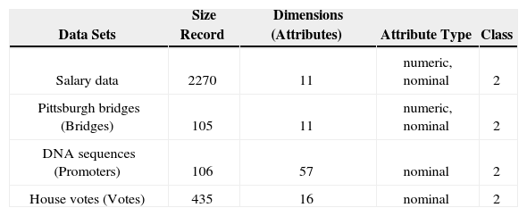
4.1Data SetsThe experiments reported here use real-world data sets to explore the feasibility of this technique for feature subset selection. These datasets are obtained from the machine learning data repository at the University of California at Irvine [19]. The experiments were performed on four datasets that are:
- 1.
Salary Data
- 2.
Pittsburgh Bridges Data
- 3.
DNA Sequences
- 4.
House Votes
The reason for choosing these data sets out of many other possibilities is that these data sets required minimum preprocessing. The characteristics of all the datasets are summarized in the Table 4. The table shows the size (number of rows) of the dataset, dimensions (total features), type of attributes (nominal and numeric) and the number of classes in the dataset.
The objective was to experiment with data sets having variations in records size and dimensions. The datasets vary in sizes such as salary data is relatively large with 2270 rows while house votes is medium sized data and the other two datasets, Pittsburgh bridges and DNA sequences are of small sizes. In the same manner the datasets vary in terms of dimensions. DNA sequences have 57 attributes while other datasets have smaller number of dimensions.
4.2PreprocessingThe data preprocessing is the first step in the experimentation. The classification algorithm is ID3 in the proposed algorithm that accepts only nominal values. For this restriction, all the continuous values are converted into nominal values. Apartfrom that missing values are handled before giving the data as input to the algorithm. All these nominal data values are then encoded in digits. This encoding is done as it simplifies the implementation of this technique.
4.2.1Conversion of Continuous Values to Nominal ValuesThe proposed feature subset selection algorithm takes the data in nominal form only. So the first step was to convert the continuous values into nominal values by defining the ranges of the continuous attribute.
Discretization techniques can be used to reduce the number of values for a given continuous attribute, by dividing the range of the attribute into intervals. These intervals can be given some label and this label is replaced by the actual data values. This research has used entropy-based discretization [9] for converting continuous attribute values into nominal values.
4.2.2Handling Missing ValuesThere were several missing values in the data sets that were needed to be handled properly. There are many options for handling the missing values such as [9]
- •
Ignore the tuple having a missing value.
- •
Fill in the missing value manually.
- •
Use a global constant to fill in the missing value.
- •
- •
Use the maximum occurring value of that attribute to fill in the missing value.
- •
Use the most probable value to fill in the missing value.
In this research for continuous value option fourth has been applied where the attribute mean has been used to fill in the missing values. For example the average income of the customers is $28,000. This value is used to replace the missing value for income. The missing values of the attributes that are nominal in nature are handled by replacing them by the most occurring value of that attribute. The most occurring value is determined by calculating the mode of all the values of that attribute. Then the missing values are replaced by that mode.After all the values are converted to nominal form and the missing values are handled properly, the next process is the encoding process. The feature subset selection in this research uses the nominal values but encoded only in digits form.
4.3Accuracy CalculationThe accuracy of the selected feature subset is calculated by applying ID3 algorithm. The data set is trimmed according to the selected feature subset. Then this trimmed data is given as input to the ID3 algorithm. The application of ID3 outputs a decision tree. This decision tree is then tested on the testing data. The testing accuracy of the tree is the accuracy (fitness) of the selected feature subset for the class under.
For the authentication of the results, 30 runs have been carried out for each experiment and the average of all the 30 runs have been reported in the results. Along with this, testing is based on 5-fold cross-validation explained in the next section.
4.4Cross-Validation for ResultsCross-validation is a method for estimating generalization accuracy based on “re-sampling” [18]. In k-fold cross-validation, the data is divided into k subsets of (approximately) equal size. The program is run k times, each time leaving out one of the subsets from training, but using only the omitted subset to compute accuracy. If k equals the sample size, this is called “leave-one-out” cross-validation. This research uses 5-fold cross-validation for the purpose of authenticating the results. The data is divided into five equal partitions in the beginning of the algorithm. Then in the evaluation function ID3 is applied five times according to the feature subset (chromosome), each time leaving out one of the partitions and using the rest of the four partitions as training data. Then the omitted partition is used as the testing data. In this manner, in the end of the evaluation function the five testing accuracies are obtained. The average of these five accuracies is measured in order to get final accuracy. This accuracy is the fitness of that particular feature subset.
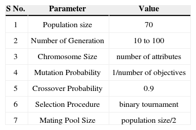
4.5Parameter Setting and ComparisonsThe population size is set to 70 as before applying 5-fold cross validation some experimentation is done by varying the population size from 20 to 100 with a jump of 10.
This experimentation showed that 70 is the appropriate population size. The number of generation size starts at 10 for each dataset and increases with an increment of 10 until the Pareto-front attains stability. The algorithm used in the feature subset selection toolbox is NSGA-II, that uses binary tournament as selection procedure and the mating pool size is set as half of the population. The crossover and mutation probabilities are set as 20% because the authors of NSGA-II have found that increasing or decreasing these probabilities results in degradation of the accuracy. The parameters for this technique are shown in Table 5.
Parameter values for the algorithm.
| S No. | Parameter | Value |
|---|---|---|
| 1 | Population size | 70 |
| 2 | Number of Generation | 10 to 100 |
| 3 | Chromosome Size | number of attributes |
| 4 | Mutation Probability | 1/number of objectives |
| 5 | Crossover Probability | 0.9 |
| 6 | Selection Procedure | binary tournament |
| 7 | Mating Pool Size | population size/2 |
This section shows the results obtained by applying the proposed technique for feature subset selection technique on the four datasets. The results are validated by 5-fold cross validation. For 5-fold cross validation the data is divided into 5 equal parts. In the evaluation function, ID3 is applied for each chromosome five times by keeping each part as the testing data and the remaining four parts as the training data. The average of all the five testing accuracies from all the five parts is taken in order to declare it as the fitness of the particular feature subset.
The improvement in the Pareto-front obtained by increasing the generation size is shown for each dataset in the form of graph. Apart from these graphs, a table is shown comparing the accuracy and the number of features with all the features included and with the selected feature subset. In the end the comparison of the proposed technique is done with one of the previous technique that treats feature subset selection ass single optimization problem.
The results have been produced using multiple datasets that are obtained from the machine learning data repository at the University of California at Irvine [19].
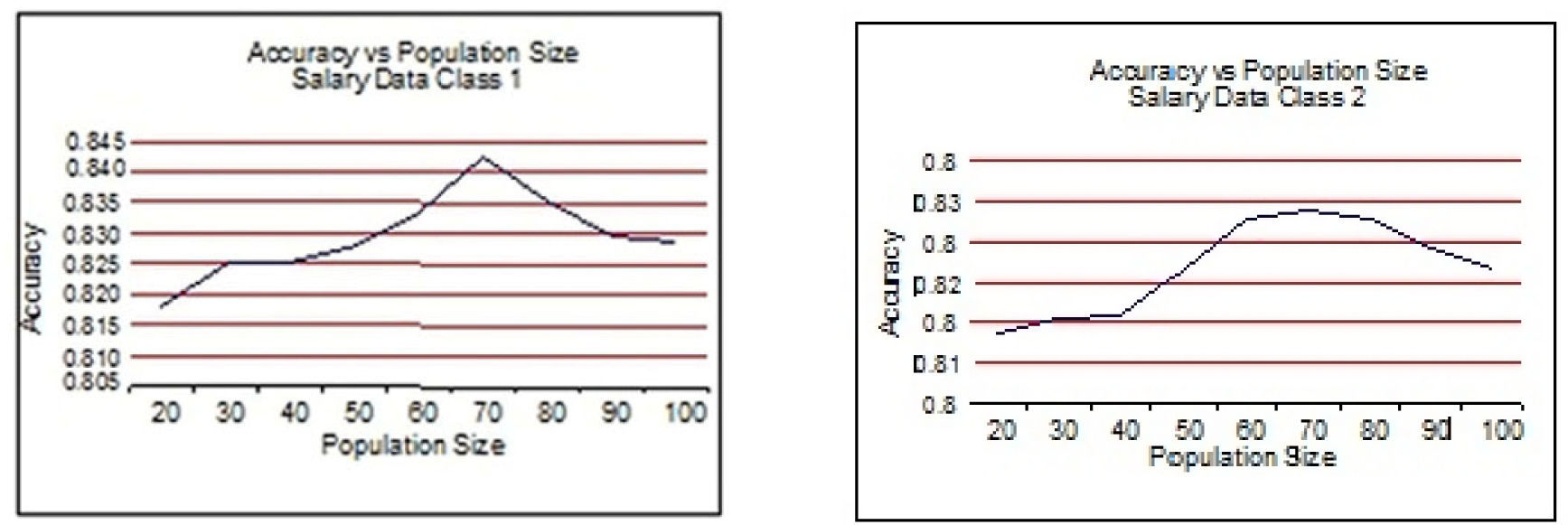
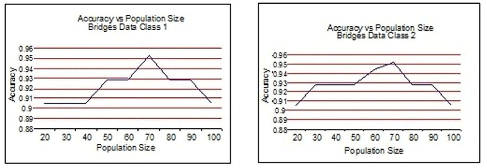
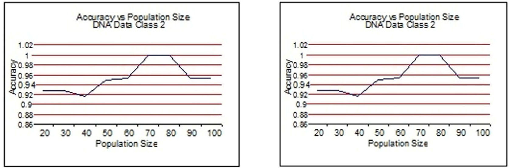
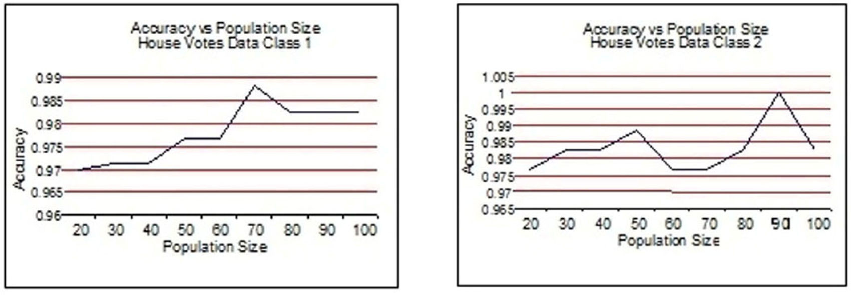
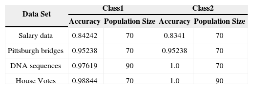
5.1Results with Different Population SizeBefore applying the 5-fold cross validation, the appropriate population size is obtained by applying the proposed feature subset selection technique on all the four datasets.
In order to achieve accuracy of the fitness value, multiple rounds of cross validation have been used. By using 5-fold cross validation, the accuracy of the fitness value of a particular solution can have multiple rounds of cross validation by using different partitions and then average of the validation results over rounds is used to have reliable measure of fitness accuracy.
For this purpose the training data is 70% of the total data and testing data is 30% of the total data. The effect of population size on all the four data sets is shown with the help of graphs. The graphs showing the accuracies by varying the population size from 20 to 100 with a jump of 10 are shown for each of the data set.
From Figure 3 to Figure 6, the accuracy of class 1 and class 2 are shown respectively for each dataset. The population size is on the x-axis and the accuracy of the respective class is on the y-axis.


This experimentation shows clearly that the proposed technique gives better results when the size of the population is 70 most of the time. This experimentation is summarized in Table 6 and on the basis of these results the population size is set to 70.
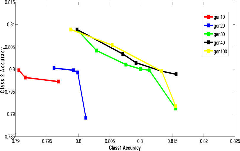
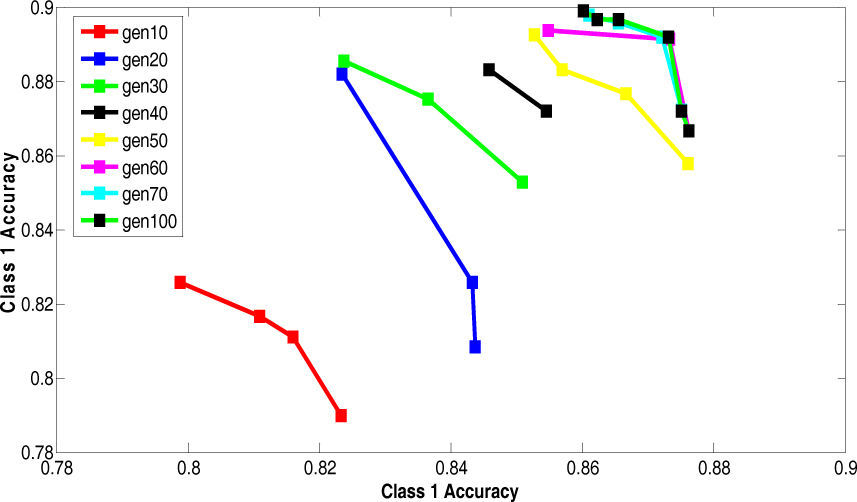
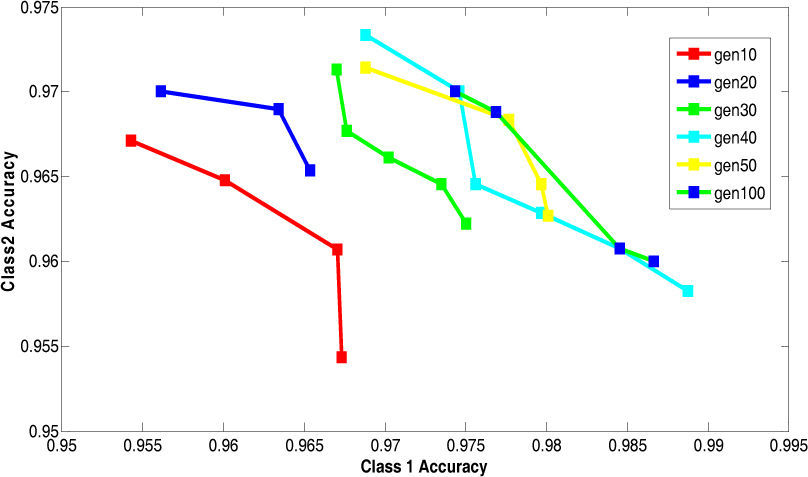
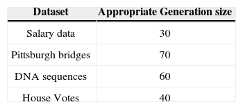
5.2Results of 5-fold Cross Validation with Different Generation SizeThis section presents the improvement in Paretofront acquired by varying the generation size and applying the proposed feature subset selection algorithm to all the four datasets. The accuracies obtained are validated by 5-fold cross validation. The population size is 70 and the rest of the parameters are same. The results are shown for the four datasets in Figure 7 to Figure 10. The accuracy of class 1 is on x-axis while the accuracy of class 2 s on y-axis. The improvement is obvious in the figures as the generation size is increased. For salary data, the Pareto-front keeps on improving until the generation size becomes 40. To validate the stability Pareto-front for generation 100 is also plotted. The Pareto-fronts of generation 30, 40 and 100 are overlapping. So, the generation size 30 provides optimal Pareto-front for salary data.


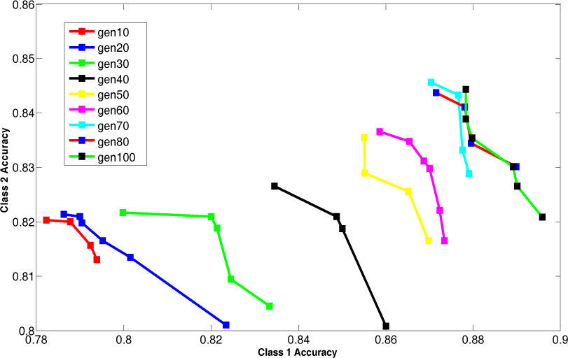
For bridges data, the Pareto-front keeps on improving until the generation size becomes 80. To validate the stability Pareto-front for generation 100 is also plotted. The Pareto-fronts of generation 70, 80 and 100 are overlapping. So, the generation size 70 provides optimal Pareto-front for bridges data.
For DNA data, the Pareto-front keeps on improving until the generation size becomes 70. To validate the stability Pareto-front for generation 100 is also plotted. The Pareto-fronts of generation 60, 70 and 100 are overlapping. So, the generation size 60 provides optimal Pareto-front for bridges data.
For house-votes data, the Pareto-front keeps on improving until the generation size becomes 50. To validate the stability Pareto-front for generation 100 is also plotted. The Pareto-fronts of generation 40, 50 and 100 are overlapping. So, the generation size 40 provides optimal Pareto-front for bridges data.
The above results are summarized in the Table 7. This table shows the appropriate generation size for each dataset.
The trend that can be easily seen is that the large number of generation size is needed for the datasets that are small in size such as bridges and DNA datasets having 106 and 105 record respectively. A small number of generation size, is needed for large datasets such as salary data having 2270 records. The same four datasets are used to create decision tree by ID3 without feature subset selection by 5 cross validation process. This process is repeated for each class separately.
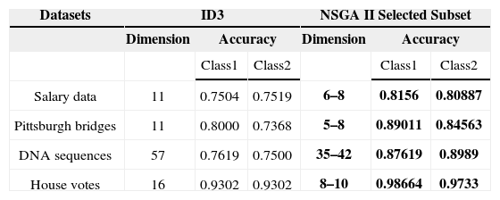
5.3Comparison of the proposed technique with simple ID3By applying the proposed technique, Pareto-front is obtained that has more than one trade-off optimal solution. The direct comparison of ID3 with the proposed technique is not possible. So for the accuracy of class 1, the feature subset considered is the one giving highest accuracy considering class 1 only. In the same manner, for the accuracy of class 2, the feature subset considered is the one giving highest accuracy considering class 2 only. If the user needs a balanced accuracy for both classes, than he can choose among other solutions in between these two. The features are reduced considerably by applying this technique.
The comparison of the accuracy of classification through this technique with the classification without feature subset selection is mentioned in Table 8. The comparison clearly indicates that the proposed technique outperforms as compared to the conventional ID3 algorithm. This technique gives higher accuracies for all the classes, decreases the number of features considerably and the user has choice of selecting the solution appropriate according to his needs. The comparison of this technique is also done with one of the previous techniques showing that this technique is a better alternative for solving feature subset selection problem.
Comparison of NSGA II with ID3.
| Datasets | ID3 | NSGA II Selected Subset | ||||
|---|---|---|---|---|---|---|
| Dimension | Accuracy | Dimension | Accuracy | |||
| Class1 | Class2 | Class1 | Class2 | |||
| Salary data | 11 | 0.7504 | 0.7519 | 6–8 | 0.8156 | 0.80887 |
| Pittsburgh bridges | 11 | 0.8000 | 0.7368 | 5–8 | 0.89011 | 0.84563 |
| DNA sequences | 57 | 0.7619 | 0.7500 | 35–42 | 0.87619 | 0.8989 |
| House votes | 16 | 0.9302 | 0.9302 | 8–10 | 0.98664 | 0.9733 |
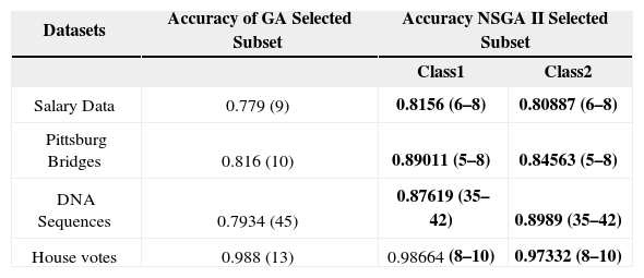
The comparison of the accuracies of the subsets selected by applying simple GA is made with this technique that applies NSGA-II and considers accuracies of different classes as separate objectives to be optimized. The results are summarized in Table 9. The accuracies obtained by simply applying ID3 with all the features are presented in Table 9. The accuracies for all the concerned datasets is shown for GA as well as NSGA-II along with the number of features indicated within braces. If we consider the accuracies for all the datasets, the proposed technique has shown considerably better results. As far as the number features are concerned the proposed technique reduces the features much more than the simple GA technique. The reduced number of features also makes the decision tree simple and more accurate. The proposed technique is a better option for feature subset selection with fewer features, higher accuracy and more than one choice of the solution for the user.
Comparison of GA selected subset and NSGA-II selected subset.
| Datasets | Accuracy of GA Selected Subset | Accuracy NSGA II Selected Subset | |
|---|---|---|---|
| Class1 | Class2 | ||
| Salary Data | 0.779 (9) | 0.8156 (6–8) | 0.80887 (6–8) |
| Pittsburg Bridges | 0.816 (10) | 0.89011 (5–8) | 0.84563 (5–8) |
| DNA Sequences | 0.7934 (45) | 0.87619 (35–42) | 0.8989 (35–42) |
| House votes | 0.988 (13) | 0.98664 (8–10) | 0.97332 (8–10) |
The results presented in this paper are obtained by applying evolutionary algorithm based technique of feature subset selection on four datasets. First of all, the appropriate population size is acquired by applying the technique on all the four datasets by varying the population size from 20 to 100 with a jump of 10. The overall results show that population size 70 is appropriate for the experimentation. Then the improvement in Pareto-front is shown by varying the generation size after applying the proposed feature subset selection algorithm to all the four datasets. The accuracies of the feature subsets are measured by 5-fold cross validation. The salary data which is the largest data of all required only 30 generations to achieve the final Pareto-front. The maximum number of generations are required by the dataset of bridges that is the smallest in terms of size.
7ConclusionThis research has used multi-objective optimization for feature subset selection for the first time. This approach is based on wrapper technique for feature subset selection. The evaluation for the candidate feature subset is measured by applying ID3 and the testing accuracy of the built tree is considered as the fitness value of that particular feature subset. The feature subset selection problem is multi-objective in nature. The accuracy of each class is an objective to be optimized. This was the basic motivation of using multi-objective genetic algorithm for solving feature subset selection problem.The experimentation is carried out on four real-life data sets. First part of the experimentation is to observe the effect of population size on the accuracies. All four of the datasets gave their best results at population size 70 to 90. Second part of the experimentation showed the effect of generation size on the Pareto-front. The authentication of results is measured by using 5-fold cross validation. The results have shown that large number of generation size is needed by small sized datasets to attain an optimal Pareto-front, while small number of generation size is required by large sized datasets. This technique makes feature subset selection non-rigid. It gives the choice to the user to choose one of the feature subsets in the Pareto-front according to his needs.
8Future WorkThe experimentation on more datasets with multiple classes will be done as a future enhancement to compare the results with other feature subset selection techniques. The future research will also include the usage of other multi-objective algorithms for solving feature subset selection problem. Few of relevant multi-objective algorithms are discussed in literature review such as Vector Evaluated Genetic Algorithm (VEGA), Aggregate by Variable Objective Weighting (HLGA), Niched Pareto Genetic Algorithm (NPGA), Non-Dominated Sorting Algorithm (NSGA) and Particle swarm optimization (MOPSO).
The comparison among the application of all these algorithms for feature subset selection problem will be carried out. The hybrid approach combining neural network and evolutionary algorithm can be used to improve the results further and to make them less conservative.
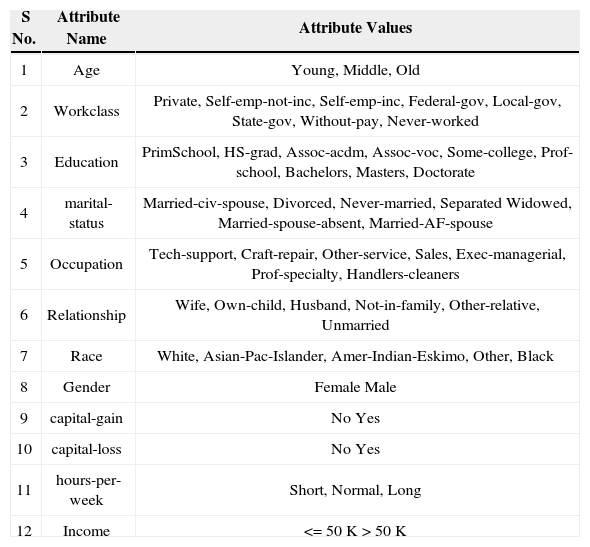
Title: UCI adult database.
Class: Income >$50k
Income <$50k based on census data
Number of instances: 2270
Number of Attributes: 11
Missing Attribute Values: none
Attribute Information:
Attribute information of salary data.
| S No. | Attribute Name | Attribute Values |
|---|---|---|
| 1 | Age | Young, Middle, Old |
| 2 | Workclass | Private, Self-emp-not-inc, Self-emp-inc, Federal-gov, Local-gov, State-gov, Without-pay, Never-worked |
| 3 | Education | PrimSchool, HS-grad, Assoc-acdm, Assoc-voc, Some-college, Prof-school, Bachelors, Masters, Doctorate |
| 4 | marital-status | Married-civ-spouse, Divorced, Never-married, Separated Widowed, Married-spouse-absent, Married-AF-spouse |
| 5 | Occupation | Tech-support, Craft-repair, Other-service, Sales, Exec-managerial, Prof-specialty, Handlers-cleaners |
| 6 | Relationship | Wife, Own-child, Husband, Not-in-family, Other-relative, Unmarried |
| 7 | Race | White, Asian-Pac-Islander, Amer-Indian-Eskimo, Other, Black |
| 8 | Gender | Female Male |
| 9 | capital-gain | No Yes |
| 10 | capital-loss | No Yes |
| 11 | hours-per-week | Short, Normal, Long |
| 12 | Income | <=50K >50K |
Title:Pittsburgh bridges
Class : Type = wooden
Type = other
Number of Attributes: 11
Missing Attribute Values: 78
Attribute Information:
Attribute information of bridges data.
| S No. | Attribute Name | Attribute Values |
|---|---|---|
| 1 | River | A, M, O |
| 2 | Location | 1 to 52 |
| 3 | Erected | Crafts, Emerging, Mature |
| 4 | Purpose | Walk, Aqueduct, RR, Highway |
| 5 | Length | Short, Medium, Long |
| 6 | Lanes | 1, 2, 4, 6 |
| 7 | Clear-G | N,G |
| 8 | Through or Deck | Through, Deck |
| 9 | Material | Wood, Iron, Steel |
| 10 | Span | Short, Medium, Long |
| 11 | Rel_L | S, S-F, F |
| 12 | Type | Suspended, Other |
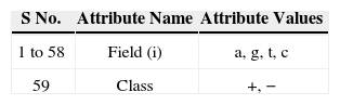
Title: E. coli promoter gene sequences (DNA) with associated imperfect domain theory
Class: positive, negative
Number of Instances: 106
Number of Attributes: 59
Missing Attribute Values: none
Class Distribution: 50% (53 positive instances, 53 negative instances)
Attribute information:
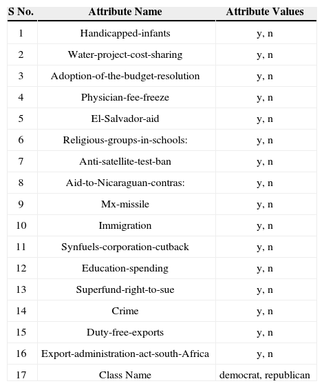
Title: 1984 United States Congressional Voting Records Database
Class: democrat, republican
Number of Instances: 435 (267 democrats, 168 republicans)
Number of Attributes: 17
Missing Attribute Values: 17
Class Distribution: (2 classes)
1. 45.2 percent are democrat
2. 54.8 percent are republican
Attribute Information:
Attribute information of house votes data.
| S No. | Attribute Name | Attribute Values |
|---|---|---|
| 1 | Handicapped-infants | y, n |
| 2 | Water-project-cost-sharing | y, n |
| 3 | Adoption-of-the-budget-resolution | y, n |
| 4 | Physician-fee-freeze | y, n |
| 5 | El-Salvador-aid | y, n |
| 6 | Religious-groups-in-schools: | y, n |
| 7 | Anti-satellite-test-ban | y, n |
| 8 | Aid-to-Nicaraguan-contras: | y, n |
| 9 | Mx-missile | y, n |
| 10 | Immigration | y, n |
| 11 | Synfuels-corporation-cutback | y, n |
| 12 | Education-spending | y, n |
| 13 | Superfund-right-to-sue | y, n |
| 14 | Crime | y, n |
| 15 | Duty-free-exports | y, n |
| 16 | Export-administration-act-south-Africa | y, n |
| 17 | Class Name | democrat, republican |