


Anisotropic Conductive Film (ACF) is essential material in LCM (Liquid Crystal Module) process. It is used in bonding process to make the driving circuit conductive. Because the price of TFT-LCD is getting lower than before in recent years, the ACF has relatively higher cost ratio. The conventional long bar ACF cutting unit is changed into short bar ACF cutting unit in new bonding technology. However, the new type machine was not optimized in process control and mechanical design. Therefore, the failure rate of new ACF cutting process is much higher than the one of the conventional process. This wastes the ACF material and rework cost is considerably large. How to make the manufacturing cost down effectively and promote the product quality is the main issue to maintain competition capability for the product. Therefore, the orthogonal particle swarm optimization (OPSO) is used to analyze the optimal design problem. The ACF cutting yield rate is selected to be objective function for optimization. The quality characteristic function for yield rate is used in orthogonal particle swarm optimization. Three control factors such as plasma clean speed, ACF peeling speed and ACF cutter spring setting are selected to study the effect of the yield rate. Results show that the proposed method can provide good optimal solution to improve the ACF cutting process for TFTLCD manufacturing process.
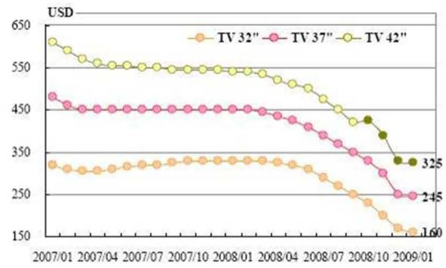
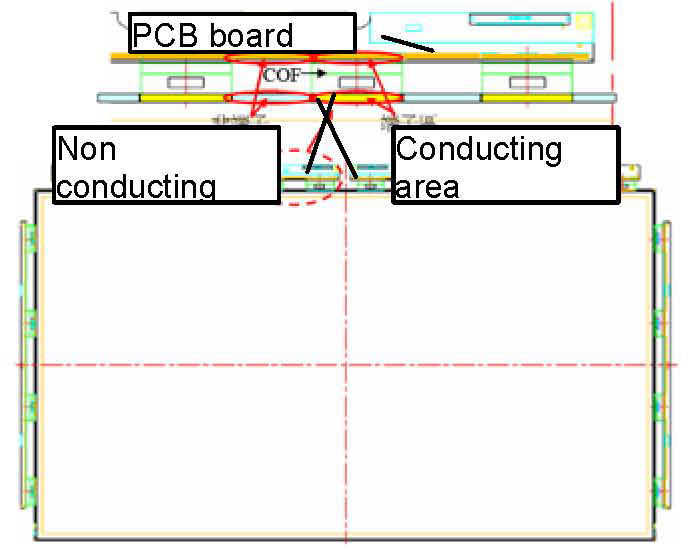
The usage amount of ACF material in global TFT-LCD industry is shown as Fig.1. It shows that the annual growth is about 13% in LCD products. The usage amount of ACF material dominates the price of LCD TV modules product. The price of LCD TV has been reduced more than 50% since 2007. Therefore, the cost of the ACF in the TFT-LCD module directly affects the profit space of TFT-LCD products. Conventionally, in long bar ACF cutting process, it is found that the nonconducting area wastes a lot of undesired ACF material. The cutting process in the LCD panel is shown in Fig. 2 [1]-[9].


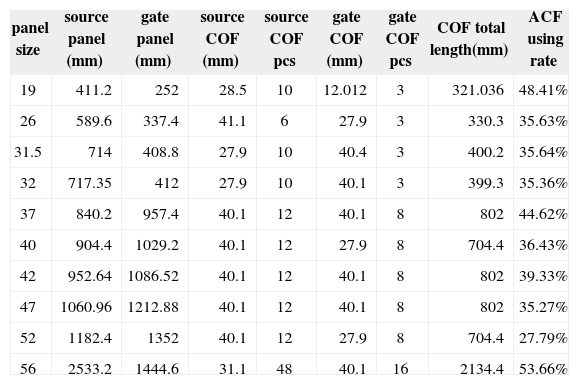
The ACF usage percentage in LCD product is shown in Table 1. The ACF usage percentage in LCD products is roughly about 35%. It means that nearly 65% of the ACF usage in cutting process is not required. This increases production cost considerably.
The usage of ACF for different size of product.
| panel size | source panel (mm) | gate panel (mm) | source COF (mm) | source COF pcs | gate COF (mm) | gate COF pcs | COF total length(mm) | ACF using rate |
|---|---|---|---|---|---|---|---|---|
| 19 | 411.2 | 252 | 28.5 | 10 | 12.012 | 3 | 321.036 | 48.41% |
| 26 | 589.6 | 337.4 | 41.1 | 6 | 27.9 | 3 | 330.3 | 35.63% |
| 31.5 | 714 | 408.8 | 27.9 | 10 | 40.4 | 3 | 400.2 | 35.64% |
| 32 | 717.35 | 412 | 27.9 | 10 | 40.1 | 3 | 399.3 | 35.36% |
| 37 | 840.2 | 957.4 | 40.1 | 12 | 40.1 | 8 | 802 | 44.62% |
| 40 | 904.4 | 1029.2 | 40.1 | 12 | 27.9 | 8 | 704.4 | 36.43% |
| 42 | 952.64 | 1086.52 | 40.1 | 12 | 40.1 | 8 | 802 | 39.33% |
| 47 | 1060.96 | 1212.88 | 40.1 | 12 | 40.1 | 8 | 802 | 35.27% |
| 52 | 1182.4 | 1352 | 40.1 | 12 | 27.9 | 8 | 704.4 | 27.79% |
| 56 | 2533.2 | 1444.6 | 31.1 | 48 | 40.1 | 16 | 2134.4 | 53.66% |
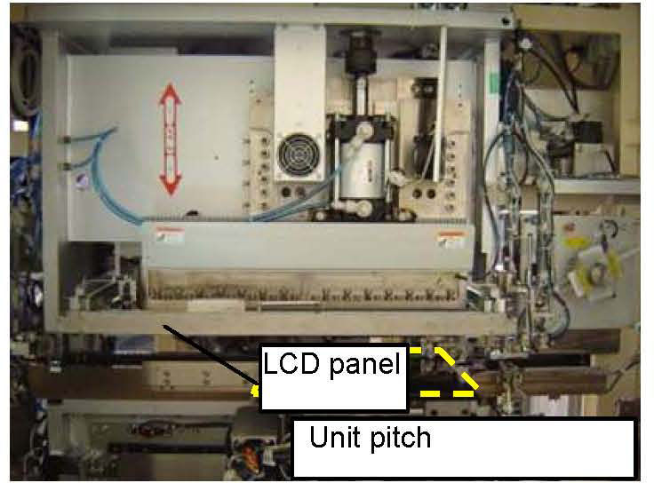
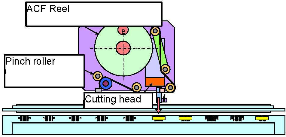
Therefore, in order to save the production cost, the design of conventional long bar ACF cutting unit in Fig. 3 has to be changed into short bar ACF cutting unit in Fig. 4.


Short bar ACF cutting method has the following advantages and disadvantages:
Advantages: 1) Since the ACF material usage is reduced, lower production cost can be achieved. 2) Since the components space placed in the PCB board is increased, more flexible manufacturing methods are provided.
Disadvantages: 1) Cutting more segments increases the tact time under the same manufacturing condition. 2) The failure rate (FR) condition (NG parts/whole cutting segments) of the short bar ACF cutting process is relatively higher than the one of the long bar ACF cutting process.
2Cutting problem description of ACF cutting processIn TFTLCD manufacturing process, there are many reasons causing failure rate (FR) in the ACF cutting process. Therefore, the peeling phenomena have to be described and defined. The state of peeling phenomena can be divided into upward peeling and downward peeling. The peeling of the location can be defined as cutting from the starting side to the end of peeling. Therefore, by peeling and cutting the ACF material in the ACF cutting process, many unexpected phenomenon possibly occurs.
From the above reasons, it seems that the bad performance of cutter actuator, the bad cutting motion, and the bad peeling condition are the three major reasons to cause the failure rate of ACF cutting process. Therefore, design of experiments (DOE) method based on response surface method (RSM) is used to improve the cleanliness of the panel and change the design condition of the cutter.
3Problem formulation using response surface methodResponse Surface Method(RSM)is generally employed to analyze and describe an unknown and complicated physical problem by design of experiments (DOE) [10]-[13]. In RSM, the mathematical analysis and statistical analysis are jointly utilized to analyze the experimental results to obtain the optimal response solution by discussing the interaction between factors.
When the RSM is employed to analyze the experimental design with a plurality of factors, the experimental runs can be further reduced to achieve the purpose of obtaining optimal solution. Accordingly, the experimental cost can be decreased.
In RSM, two kinds of response surfaces are discussed and defined:
- a)
Average response surface EZ (y(x,z)): it represents the average value of a response surface y(x,z) with control factor vector x and noise factor vector z.
- b)
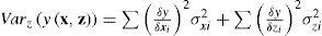
Variance response surface Varz (y(x,z)) : it represents the variance of a response surface y(x,z) with control factor vector x and noise factor vector z.
Some advantages of RSM are described as follows:
- a)
Not only the average response is evaluated, but also the variance response is evaluated.
- b)
Both of the average response and variance response are considered to optimize the response surface.
The concept of the RSM is to define the response surfaces of average and variance individually. Therefore, the two response surfaces may be separately analyzed independently. However, the RSM might have trade-off problem between the two response surfaces. The trade-off problem is formulated by using optimization. With the definition of objective function and constraints, the trade-off problem can be solved by using optimization process.
Therefore, the RSM is quite different from the Taguchi method which only uses one index, the SN ratio, to analyze optimal design.
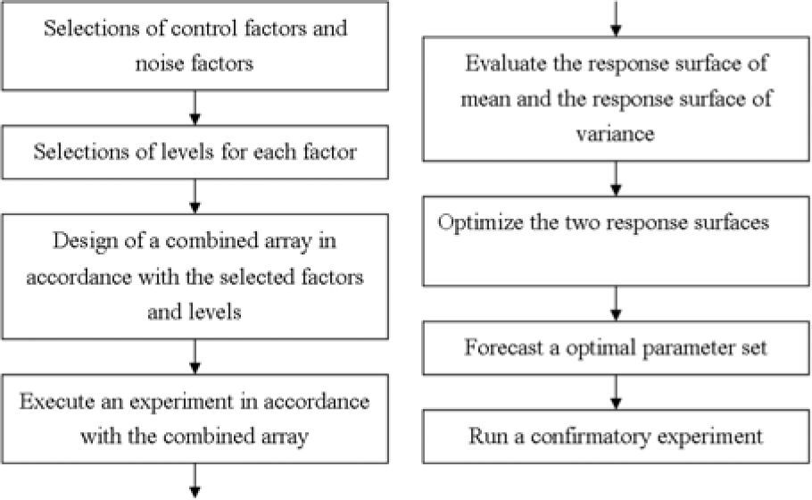
The RSM consists of design steps as follows:
- 1)
Design a combined array in accordance with selected factors and levels
- 2)
Evaluate the average response surface and the variance response surface.
- 3)
Optimize the two response surfaces using OPSO process.
The design flow chart of the RSM is shown in Fig. 5.6.
3.1Design of combined arrayThe weakness of Taguchi method is that the average and variance are defined together in a mixed way. A better strategy is to design the combined array with high enough resolution that incorporates both the control factors and noise factors by using response surface method. The average and variance can be discussed separately.
3.2Definition of two response surfacesIn most of the optimal design case, the relation between the response and independent variables is usually unknown. Therefore, in RSM, the first step is to find a suitable formulation to describe the adequate relation between the response and the considered independent variables. If the response can be modeled by a regressive model with lower curvature, the response can be modeled by a first-order model.
The average response can be modeled by using regressive analysis. The response function for first-order or second-order regressive model can be formulated by

where
x: vector of controllable factors;
z: vector of uncontrollable factors, or called the noise factors;
b0 : term of constant;
b: coefficients of the vector of controllable factors;
b: matrix of the interacted term between controllable factors;
c: coefficients of the vector of uncontrollable factors;
K: matrix of the interacted term between controllable factor and uncontrollable factor;
x’b: linear term of controllable factors;
x’bx: interaction term between controllable factors;
z’c: linear term of uncontrollable factors;
x’kz: interaction term between controllable factor and uncontrollable factor;
After finding the response surface y(x,z), the average response surface EZ(y(x,z)) and variance response surface Varz(y(x,z)) have to be evaluated by the response surface y(x,z).
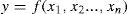
The two response surfaces can be modeled by using error propagation theory. If y is a function of plural controllable factors including x1,x2…,xn That is, the function y can be represented as
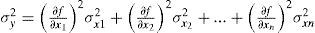
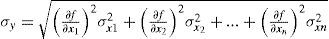
The average value µy variance σy2, and standard deviation σy of the function y are further formulated as follows:

In the following, how to model the two response surfaces by using the error propagation theory is discussed. The following assumptions should be discussed in advance.
a) Assumption 1: σx2=0 for each controllable factor
In design of experiments (DOE) method, three levels for each controllable factor can be selected to evaluate the optimal problem. Therefore, the system variance impacted by each controllable factor should be zero. That is to say, no variance exists among the controllable factors since they are controllable.
b) Assumption 2: σz2=1 and µz = 0 for each noise factor
The noise factor is generally an uncontrollable factor, since the noise often unexpectedly occurs in the system. Therefore, the system variance impacted by each noise factor unavoidably exists in the system. To simplify the modeling, both the control factors and noise factors can be transformed into the coded normalized variables for natural variables, ξ.The coded procedure includes the following steps:
1) Estimate the average value ξ¯ and the standard deviation σξ of the natural variable.
2) Code and normalize the natural variable by using (ξ−ξ¯σξ).
After coding, the average value and the standard deviation of the noise factor are μz = 0 and σz2=1. That is to say, no average value exists among the noise factors. The standard deviation is normalized to be 1.
The mentioned two assumptions are considered based on error propagation theory to further establish the following two response surfaces.
1) Establish the average response surface
From Eq. (5.38), the average value of Eq. (5.37) can be represented as

Referring again to assumption 2, the average value of the noise factor is set to zero z=0. Therefore, the Eq. (5.41) can be rewritten

2) Establish the variance response surface
By using the error propagation theory, the response surface of variance can be represented as
Referring again to assumption 1, the variance of the control factor is set to zero σx2=0. Therefore, the Eq. (5. 43) can be expressed as:
4System formulation of cutting process using response surface method
Dual response surfaces method is used to formulate the optimization problem. Based on response surface method, the average response surface and variance response surface have to be found first. The optimization problem is to maximize the objective function formulated by average response surface subject to constraint condition formulated by the variance response surface. In order to verify the validity of the optimization process and find optimal solution set, testing case is illustrated in the following.
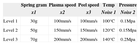
The central point experiment means that the spring gram elastic constant is 50 g. The plasma cleaning velocity is 150 mm/s. The cutter peeling speed is 150 mm/s. The three control factors and two noise factors defined for response surface method are shown in Table 2.
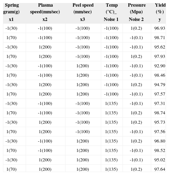
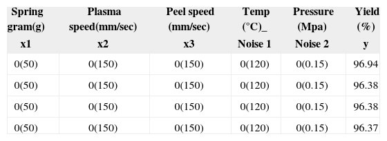
The combinational array is listed in Table 3 for the response surface method. The temperature and pressure are selected as noise factors. The experimental runs of the yield rate values for the ACF cutting process for are listed in Table 3. Besides, the four central point repeated experiments are required to be measured in Table 4.
Combinational Array in Response Surface Method.
| Spring gram(g) | Plasma speed(mm/sec) | Peel speed (mm/sec) | Temp (°C)_ | Pressure (Mpa) | Yield (%) |
|---|---|---|---|---|---|
| x1 | x2 | x3 | Noise 1 | Noise 2 | y |
| -1(30) | -1(100) | -1(100) | -1(100) | 1(0.2) | 96.93 |
| 1(70) | -1(100) | -1(100) | -1(100) | -1(0.1) | 98.71 |
| -1(30) | 1(200) | -1(100) | -1(100) | -1(0.1) | 95.62 |
| 1(70) | 1(200) | -1(100) | -1(100) | 1(0.2) | 97.93 |
| -1(30) | -1(100) | 1(200) | -1(100) | -1(0.1) | 92.90 |
| 1(70) | -1(100) | 1(200) | -1(100) | -1(0.1) | 98.46 |
| -1(30) | 1(200) | 1(200) | -1(100) | 1(0.2) | 94.79 |
| 1(70) | 1(200) | 1(200) | -1(100) | -1(0.1) | 97.57 |
| -1(30) | -1(100) | -1(100) | 1(135) | -1(0.1) | 97.31 |
| 1(70) | -1(100) | -1(100) | 1(135) | 1(0.2) | 98.74 |
| -1(30) | 1(200) | -1(100) | 1(135) | 1(0.2) | 95.73 |
| 1(70) | 1(200) | -1(100) | 1(135) | -1(0.1) | 97.56 |
| -1(30) | -1(100) | 1(200) | 1(135) | 1(0.2) | 96.80 |
| 1(70) | -1(100) | 1(200) | 1(135) | -1(0.1) | 98.52 |
| -1(30) | 1(200) | 1(200) | 1(135) | -1(0.1) | 95.02 |
| 1(70) | 1(200) | 1(200) | 1(135) | 1(0.2) | 97.64 |
Combination table and experiment results for the four central point experiments.
| Spring gram(g) | Plasma speed(mm/sec) | Peel speed (mm/sec) | Temp (°C)_ | Pressure (Mpa) | Yield (%) |
|---|---|---|---|---|---|
| x1 | x2 | x3 | Noise 1 | Noise 2 | y |
| 0(50) | 0(150) | 0(150) | 0(120) | 0(0.15) | 96.94 |
| 0(50) | 0(150) | 0(150) | 0(120) | 0(0.15) | 96.38 |
| 0(50) | 0(150) | 0(150) | 0(120) | 0(0.15) | 96.38 |
| 0(50) | 0(150) | 0(150) | 0(120) | 0(0.15) | 96.37 |
For the four repeated experimental values, the average value is calculated as:

For the experimental data in combinational array, the average value is also computed as:

The sum of variance for the curvature is:

The sum of variance for the error is:

The F-statistic value is calculated as:
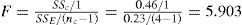
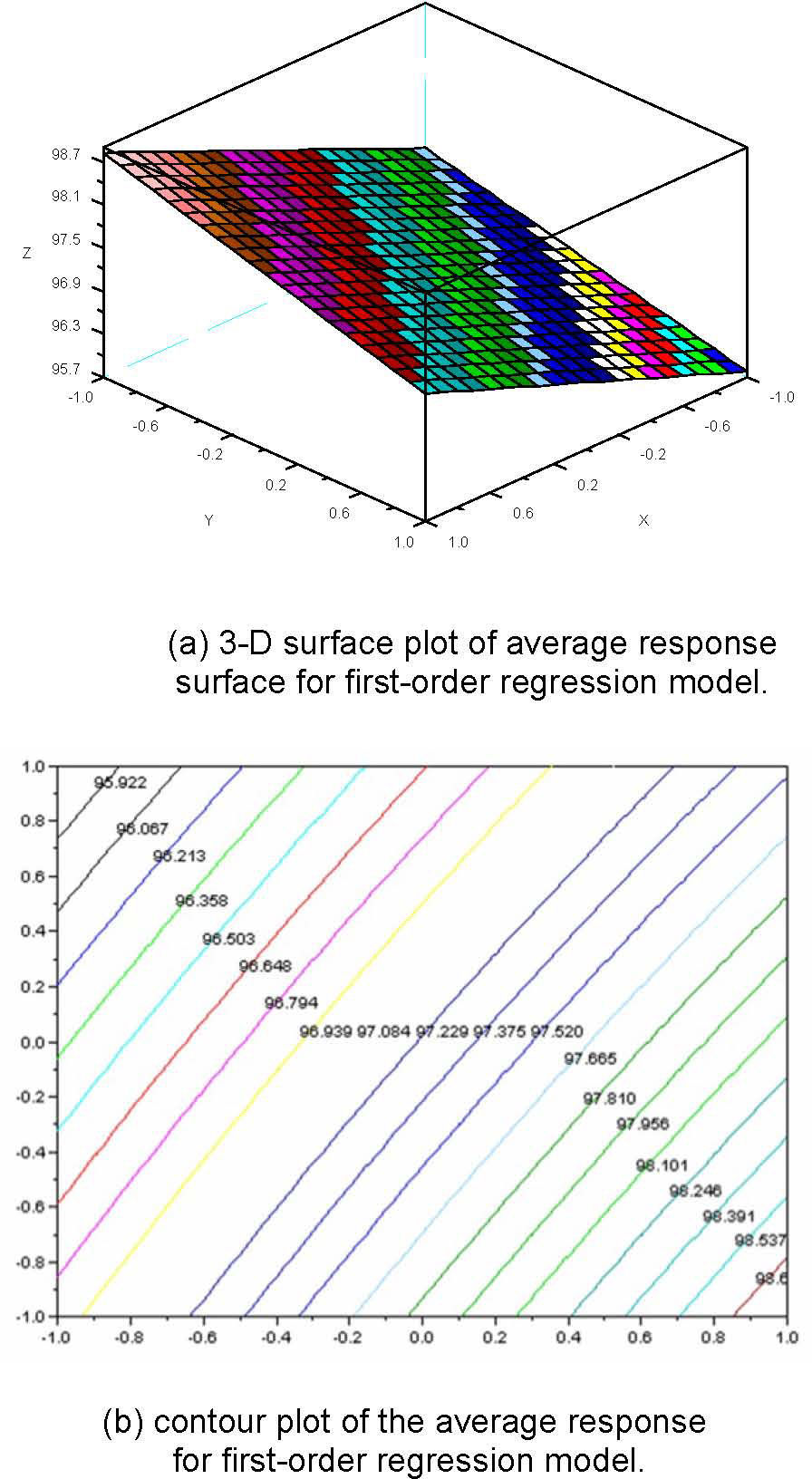
It shows that the curvature is not large. Therefore, it is suitable to use the first-order regressive model. The derived average response surface is computed as:
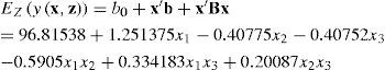
The corresponding 3-D surface plot and contour plot are shown in Fig. 5.

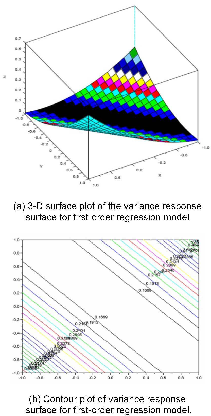
The variance response surface is derived as:


If the standard deviation for z1, z2 is set to σz1=1, σz2=1 respectively,
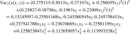
The corresponding 3-D surface plot and contour plot are shown in Fig. 6.

Therefore, the variance response surface is used to be the constrained condition for the optimization problem.
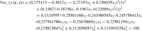
where the following inequalities should be satisfied.
5Orthogonal particle swarm optimization process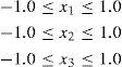
With the above derived system model by response surface method, the optimization process is performed to derive the optimal solution set for this problem. However, the optimal solution may be located anywhere in the range of -1.0 and +1.0. The local optimal solution may not be the optimal in the global region. Therefore, the OPSO process is used to derive the optimal solution in an efficient way. The local searching and global searching are going simultaneously. Global optimal solution can be found.
By adding the random seeds into formulation, the OPSO can jump out of the local optimal solution if the global solution is more optimal than the local solution. In the following, the OSPO formulation is performed. Since in the response surface method, the nonlinear problem is formulated as first-order model problem. However, the curvature for this model is large. That means the nonlinearity property is still heavy in this problem. This influences the searching process when finding the optimal solution.
The particle swarm optimization originates from the emulation of the group dynamic behavior of animal. For each particle in a group, it is not only affected by its respective particle, but also affected by the overall group. There are position and velocity vectors for each particle. The searching method combines the experience of the individual particle with the experience of the group. For a particle as a point in a searching space with D-dimensional can be defined as [14]-[19].
The i-th duty cycle particle associated with the MPPT controller can be defined as:

where d=1,2,…,D and i=1,2,…,PS, PS is the population size. The respective particle electric power and group electric power associated with each duty cycle Xid are defined as:
The refreshing speed vector can be defined as

The refreshing position and velocity vectors can be expressed as
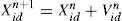
When the searching begins, the initial solution is set. In the iteration process, the particle is updated by the value coming from group duty cycle and particle duty cycle. The convergence condition is dependent on the minimum of the average square error of the particle. Both the experience of the individual particle and the experience of the group are mixed into the searching process.
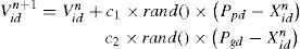
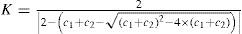
In the optimization problem, there might be a local minimum problem. The optimal solution might jump into a local trap and can not jump out of the trap. Actually, a local minimum point does not represent a global solution in a wide range. In the group experience, random function is used to jump out of the local interval. An inertia weighting factor is considered in this algorithm to increase the convergence rate. An inertia weighting factor is added in the following expression. The modified formula can be expressed as:
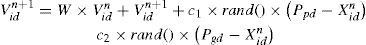
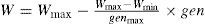
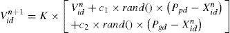
where the C1 and C2 are both constants. Wmax is The initial weighting value. Wmin is the final weighting value. gen is the number of current generation. genmax is the number of final generation. However, the above mentioned is actually a kind of linear modification. To make the algorithm suitable for nonlinear searching problem, there is many nonlinear modification methods proposed to refresh the velocity vector. The modified term is defined as the key factor. By setting the learning factors c1 and c2 which are larger than 4.0, the modification for the speed vector is expressed as:
A modified PSO method called orthogonal PSO (OPSO) is proposed to solve the update problem effectively. A simple orthogonal array in Taguchi method is used in this algorithm to help the update.
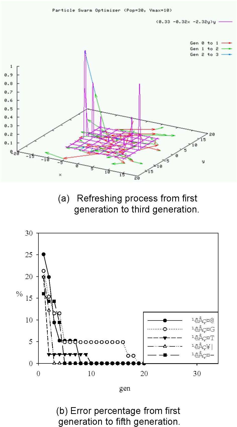
6Orthogonal array algorithm in OPSO methodTo run the Taguchi method, two functions are defined first. The particle swarms are composed of individual particle swarm Oid and group particle swarm Aid.
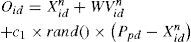

These two functions are specified as two control factors in Taguchi method. Two levels are defined for the control factors. Therefore, the orthogonal array has two factors and two levels. The electric power calculating from the MPPT converter is used as the measured value in orthogonal array. Assume that the optimal solution is expressed as Qid. The Qid is adopted to refresh the particle position and velocity vectors as shown in the following expression. The particle refreshing process in OPSO optimization is illustrated in Fig. 7.
7Discussion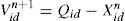


This paper has achieved the aim of finding optimal solution for the TFTLCD manufacturing process. The derived optimal solution can provided the manufacturing process under the optimal operating condition.
By using the response surface method with OPSO method, the mathematical model for this problem is provided and verified. This will be very helpful to associated industrial application.
The optimal solution can be found and located at the ends of the range. Global solution is found instead of local solution. Results show that the proposed mathematical method has the capability of finding appropriate searching process.
8ConclusionThrough the analysis of response surface method combined with OPSO process, the optimal solution is found. The optimal solution is located at (x1,x2, x3)=(0.98, −0.97, −0.98).
The corresponding optimal solution for yield rate is 99.30. The local optimal solution is avoided and the proposed OPSO algorithm can find the optimal solution at the endpoints globally. In OPSO, global and local optimal ranges are searched at the same time. The related confirmation experiments show that the proposed methodology can provide good prediction with the practical case.
It is convinced that the proposed optimal parameter solution solved by OPSO algorithm can increase the cutting yield rate of ACF cutting process for the TFT-LCD module.

The authors would like to thank Chi-Mei Inc. for providing the required testing equipment. The editing help by Tzeng Tseng is also appreciated.