


Estimation of distribution algorithms (EDAs) constitute a new branch of evolutionary optimization algorithms that were developed as a natural alternative to genetic algorithms (GAs). Several studies have demonstrated that the heuristic scheme of EDAs is effective and efficient for many optimization problems. Recently, it has been reported that the incorporation of mutation into EDAs increases the diversity of genetic information in the population, thereby avoiding premature convergence into a suboptimal solution. In this study, we propose a new mutation operator, a transpose mutation, designed for Bayesian structure learning. It enhances the diversity of the offspring and it increases the possibility of inferring the correct arc direction by considering the arc directions in candidate solutions as bi-directional, using the matrix transpose operator. As compared to the conventional EDAs, the transpose mutation-adopted EDAs are superior and effective algorithms for learning Bayesian networks.
Estimation of distribution algorithms (EDAs) constitute a new branch of evolutionary algorithms for machine learning and data mining, more recently, optimization techniques [1,2,3]; their basic workflow is identical to that of genetic algorithms (GAs), which repeat a set of genetic operations (e.g., selection, crossover, and mutation) until a stopping criterion (e.g., the number of generations, a running time, and a specific fitness value) is satisfied [4,5,6]. The distinction between EDAs and GAs is based on the manner in which the genetic information is reproduced for offspring. GAs rely on crossover and mutation operators to generate offspring from two or more individuals, whereas EDAs use a probabilistic model estimated from the selected individuals. The advantages of EDAs over GAs are the absence of variation operators to be tuned and the expressiveness of the probabilistic model that drives the search process. Owing to these advantages, EDAs have been widely used as intuitive alternatives to GAs. EDAs can be grouped according to the manner in which they address dependencies among variables: independence among all variables (Univariate Marginal Distribution Algorithm (UMDA), Population-Based Incremental Learning (PBIL), Compact Genetic Algorithm (cGA)), pairwise dependencies (Mutual Information Maxminization for Input Clustering (MIMIC), Bivariate Marginal Distribution Algorithm (BMDA), Dependency-Trees based EDA (DTEDA)), and multiple dependencies (Extended Compact Genetic Algorithm (EcGA), Estimation of Bayesian Networks Algorithm (EBNA), Bayesian Optimization Algorithm (BOA)).
With regard to Bayesian structure learning, Blanco et al. [7] first used EDAs to learn the structure of Bayesian networks, and they showed that the results yielded by EDAs were superior to those yielded by GAs. It has been proved that the heuristic scheme of EDAs is effective and efficient for learning Bayesian networks. Recently, it has been reported that the incorporation of the mutation operator in EDAs can increase the diversity of genetic information in the generated population [8,9,10,11]. The incorporation of bitwise mutation makes it possible to avoid premature convergence to a sub-optimal solution, especially when the population size is not sufficiently large or if an initial population bias exists; its effectiveness has been shown in several optimization problems such as the Onemax function, the four-peaks problem, and the max-sat problem. However, the effectiveness of mutation-based EDAs in terms of the structure learning of Bayesian networks has not been investigated extensively.
We first present a new mutation operator, a matrix transpose, specifically designed for Bayesian structure learning; a matrix transpose mutation is a closed operator when the Bayesian network is described by a matrix representation. A transpose mutation enhances the diversity of the offspring and increases the possibility of inferring the correct arc direction by considering the direction of edges in candidate solutions as bi-directional.
By exploiting a transpose mutation, we investigate the extent to which the performance of EDAs can be improved, and we try to determine the most improved EDA algorithm for learning Bayesian networks. To the best our knowledge, this study involves the first such comparison of EDAs with mutation for Bayesian structure learning. To this end, we compare the performance of four standard EDAs with that of their mutation-adopted versions; the bitwise and transpose mutation versions are tested. Section 2 briefly provides background information on the EDAs. Section 3 describes the issues of EDAs associated with mutations and presents the proposed transpose-adopted EDAs. Section 4 highlights the potential of the proposed approach through various experimental examples. Concluding remarks are presented in Section 5.
2Related workThe basic workflow of EDAs is similar to that of conventional GAs. After randomly reproducing chromosomes for the first generation, it repeats a set of genetic operations, i.e., selection, estimation, and reproduction, until a stopping criterion is fulfilled. A new population of individual solutions is generated by sampling a probabilistic model, which is estimated on the basis of representative individuals selected from the previous population. The dependencies among variables in each individual are expressed by the joint probability distribution of the individuals selected at each generation.
Because the solutions of EDAs are evolved through a probabilistic model, the main issue is the construction of an effective probabilistic model. Many studies have proposed a variety of probabilistic models; they can be categorized into three approaches according to the manner of capturing the dependencies among variables: univariate, bivariate, and multivariate approaches.
The univariate model is based on the assumption of independence among variables; it factorizes the joint probability of the selected individuals as a product of univariate marginal probabilities. UMDA uses the simplest approach to estimating the joint probability distribution [13]; each univariate marginal distribution is estimated from the marginal frequencies of the selected individuals. In contrast, PBIL uses the probability distribution of the previous generation, in addition to that of recently sampled individuals, to calculate a new probability distribution [14]. The cGA is a tournament-based incremental algorithm; it updates the probability distribution using the winner of two competing individuals [15].
Bivariate EDAs consider the dependencies among pairs of variables by using efficient data structures. MIMIC searches for the best permutation among variables by using a chain structure to capture the pairwise dependencies among the variables [16]. BMDA factorizes the joint probability distribution for second-order statistics by using an acyclic dependency graph [17]. DTEDA uses a tree structure to represent dependency relationships [18].
Multivariate EDAs factorize the joint probability distribution by using statistics of order greater than two. The probabilistic model complexity and the computational cost of determining the model are greater than those in the cases of univariate and bivariate EDAs. Thus, such approaches require a more complex learning process. EcGA divides the variables into a number of groups, and then factorizes the joint probability distribution as a product of marginal distributions of variable size [19]. EBNA uses the Bayesian information criterion (BIC) score to learn the joint probability model of the selected individuals [20]. BOA uses the Bayesian Dirichlet equivalent (BDe) measure to compute the quality of each candidate dependency [21].
Bayesian networks are graphical structures for representing the probabilistic relationships among variables [22]. The structure learning of Bayesian networks is an NP-Hard optimization problem because the number of structures grows exponentially with the number of variables [23]. It has been shown that the heuristic approach of EDAs is effective and efficient because of the extremely high cardinality of the search spaces. With regard to the application of EDAs for learning Bayesian networks, Blanco et al. used the UMDA and PBIL to infer the structure of Bayesian networks [7]. MIMIC was used to obtain the optimal ordering of variables for Bayesian networks [24]. The Bayesian networks learned using UMDA, PBIL, and MIMIC were more accurate than those learned using GAs, as compared to the original networks.
3Proposed method3.1RationaleAs mentioned previously, EDAs assume that it is possible to build a probabilistic model of the promising areas of the search space, and they use this model to drive the search for the optimum solution. To validate this assumption, it is important to maintain the diversity of individuals in the generated populations in order to avoid premature convergence to a sub-optimal solution. For example, the search space for EDAs can be reduced to only those solutions that are locally optimal with respect to the probabilistic model when the population size is not sufficiently large or when an initial population bias exists; the absence of genetic operators makes it difficult to explore the uncharted search space in next generations.
Recent studies have proposed new EDAs that employ mutation operators in standard EDAs to increase the population diversity. Handa used a bitwise mutation in UMDA, PBIL, MIMIC, and EBNA [8]; it was shown that the mutation operator improved the quality of solutions for the four-peaks problem, Fc4 function, and max-sat problem. Gosling et al. used a guided mutation in PBIL for the IPD strategy problem [9]; the mutation operator constrained the variation to solutions that were shown to be effective in the previous generation. Heien et al. compared the effectiveness of the bitwise mutation operator in BOA [10]; the mutation increased the success rate and reduced the minimum required population size in four function problems (Onemax, 5-trap, 3-deceptive, and 6-bipolar). Pelikan et al. analyzed the effects of bitwise mutation on improving the performance of UMDA through two test problems (Onemax and noisy Onemax) [11].
The benefits of mutation-based EDAs have inspired some researchers to investigate the effectiveness of mutation-based EDAs in learning the optimal structure of Bayesian networks. Furthermore, conventional bitwise mutations are not closed operators from the viewpoint of the acyclicity of Bayesian networks; they can generate illegal solutions with cycles. Thus, in this study, we investigate the effectiveness of mutation-adopted EDAs in identifying an optimal Bayesian network structure. To this end, we propose a new mutation operator, a transpose mutation, designed for Bayesian structure learning; it enhances the diversity of offspring and increases the possibility of inferring the correct arc direction by considering the arc directions in candidate solutions as bidirectional, using a matrix transpose operator.
3.2Matrix transpose mutationWhen developing a mutation operator, it is often recommended that small variations should be used to engender small changes in the resulting offspring’s quality [25]. From this point of view, we find that a bitwise mutation in Bayesian Networks can greatly impact the offspring’s quality because it introduces new random arcs between nodes that were not considered in the probable solutions. Therefore, we tried to design a mutation operator to work within the current form of nodes and arcs in a candidate solution. To achieve this, we propose a matrix transpose mutation that generates offspring by inverting arcs in the current probable network. This variation can inherit informative information from previous solutions to guide the search over the probable solution space, and explore new states for offspring by changing the direction of arcs. By considering the arc as bi-direction, the candidate solutions are evolved by reproducing arcs for new offspring based on a probability distribution with contributions from all arcs to infer the most probable arc direction probabilistically.
In general, the choice of variation operators should follow intuitively from the problem representation. To introduce randomness that was not considered in the probable solutions, we propose a matrix transpose mutation that is appropriate for a matrix representation. The operator generates offspring by inverting the arc direction in the individuals, which can inherit the information of solutions to drive the search over probable solutions and explore new states for offspring by changing the arc directions.
To represent a Bayesian network, we use a matrix representation, the most intuitive representation of a Bayesian network (an individual chromosome). We represent a network as an n×n connectivity binary matrix M. The matrix element M(i,j) in row i and column j is 1 if and only if variable i is a parent of variable j in the network. For example, the network in Fig. 1 (left) is represented in matrix form in Fig. 1 (right).

On the basis of the matrix representation, we build a probability matrix P that indicates the probability distribution of arcs among nodes in the selected individuals; it estimates the probability distribution of dependencies among variables.
Definition (Probability Matrix). Let M={M1, M2, …, Md} be a given population of individuals (networks). Let S={S1, S2, …, Sh} (S ⊆ M) be a subset of representative individuals selected from M using their fitness ranks. Then, the n×n binary matrix P is defined by estimating the probability distribution of S. The matrix element P(i,j) in row i and column j is 0 when i and j are equal; otherwise, it is defined as:
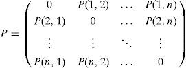
where

To construct P, a set of individuals (S) is selected according to the ranking of their fitness scores. Using h individuals, the occurrence frequency, and the average of each arc linking two nodes i and j, P(i,j) is calculated as shown in Eq. (2).
Hence, each P(i,j) (0≤P(i,j)≤1) represents the frequency with which an arc occurs in the selected individuals that were evaluated as promising individuals, and the importance of the arc in constructing an optimal structure.
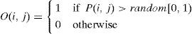
For the next generation, the offspring O is generated by the probability matrix and transpose mutation until the number of offspring becomes d.
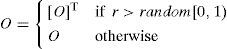
To generate an element O(i,j) of an offspring O, two probability values, i.e., P(i,j) and a random number, are compared. Specifically, the element O(i,j) is assigned a value of 1 if P(i,j)>random[0,1); otherwise, it is assigned a value of 0.
In the case of a matrix representation, a variation operator has the choice of reversing the direction of arcs between two nodes with a simple matrix transpose; it replaces O(i,j) with O(j,i) according to a mutation rate (r). Specifically, the element O(i,j) is assigned a value of O(j,i) if r>random[0,1); otherwise, it is assigned a value of O(i,j).

Fig. 2 shows the resulting matrix of an offspring before and after the transpose mutation, Obefore and Oafter, respectively.
 and after (right) a matrix transpose operator.")
The matrix transpose mutation follows intuitively from the matrix representation, while preserving the necessary properties of the matrix, and it explores the conditional dependencies among variables in reverse order. A reversal operator has been widely used for the traveling salesman problem because of the possibility of avoiding local optima [25]. Moreover, the matrix transpose is a closed operator under Bayesian structure learning; illegal networks with cycles are not reproduced.
3.3AlgorithmThe following steps show an example of the process of the proposed method. Let us suppose that the desired optimal structure is shown in Fig. 1, and the randomly generated initial population is composed of four individuals (Fig. 3). Let the number of variables, size of the population, and number of selected individuals be n=4, d=4, and h=2, respectively; the two selected individuals are S1=M1 and S2=M3.

Then, the steps of the algorithm can be described as follows:
Step 1: Generate d individuals for the first population.
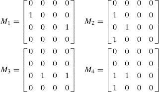
Step 2: Select h individuals by a fitness function, say S1=M1 and S2=M3.
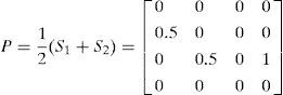
Step 3: Estimate a probabilistic model P for h individuals.
Step 4: Generate a new offspring O.

Step 5: Alter O by the transpose mutation using mutation rate (r).
Step 6: Generate d new individuals by repeating Steps 4~5.
Step 7: Repeat Steps 2~5 until the stopping criteria are satisfied.
Let us suppose that the value of random[0,1) is set to 0.1 in Steps 4 and 5; then, we obtain the first new offspring (O1) shown in Fig. 4 (left). In Step 5, if O1 is transposed under mutation r=0.2, then O1 becomes the optimal structure seen in Fig. 1:
4Result4.1Data sets and implementation parameters and after (right) a matrix transpose operator.")
To test the mutation-adopted EDAs, we applied four EDAs as well as their mutation-adopted versions to two widely used data sets, and we compared the performances of the algorithms. We employed two previous mutations; the bitwise mutation and the guided mutation [12].
The standard EDAs were UMDA, PBIL, MIMIC, and BOA; the bitwise mutation versions were UMDA+B, PBIL+B, MIMIC+B, and BOA+B; the guided mutation versions were UMDA+G, PBIL+G, MIMIC+G, and BOA+G; and the transpose mutation versions were UMDA+T, PBIL+T, MIMIC+T, and BOA+T.
The data sets employed were the Diabetes and Asia data; they have been widely used for comparative purposes in Bayesian structure learning. The Diabetes data set is a diagnostic network for predicting the signs of diabetes [26]. The Diabetes network contains nine variables and 11 arcs. The Asia data set contains the relevant variables and relationships for medical knowledge related to the shortness of breath (dyspnoea) [27]. The network contains eight variables and eight arcs. Each network was used to generate sample cases, each of which contains 10,000 instances.
In these experiments, the well-known BDe and MDL scores for Bayesian networks were used as the fitness function [22, 23]. The additional parameters were set as follows. The number of generations was set to 400; various mutation rates were used (r=0, 0.01, 0.05, 0.1, 0.15, 0.2); five population sizes were used (d=10, 50, 100, 150, 200); and five values of the learning parameter of the PBIL were used (a=0.1, 0.3, 0.5, 0.7, 0.9).
Therefore, we designed 16×2×5×5×5 (16 EDAs, 2 fitness scores, 5 populations sizes, 5 mutation rates, and 5 learning parameters) tests, and for each of these 4,000 configurations, we use 2 data sets, which gives us a total of 8,000 experiments. Each experiment was run 30 times.
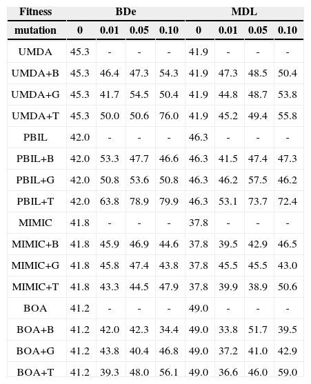
4.2Performance ComparisonTables 1 and 2 list the precisions achieved by each EDA for the two data sets for r=0, 0.01, 0.05, and 0.1 (with d=50 and a=0.5 fixed). The precision is the fraction of inferred arcs that are relevant to the network, which were assessed by comparing the network inferred by the EDAs with the original network; a higher value of precision indicates a better learning result, with perfect learning yielding a value of 100.0%.
Comparison of precision (%) achieved by EDAs for the Diabetes data.
| Fitness | BDe | MDL | ||||||
|---|---|---|---|---|---|---|---|---|
| mutation | 0 | 0.01 | 0.05 | 0.10 | 0 | 0.01 | 0.05 | 0.10 |
| UMDA | 45.3 | - | - | - | 41.9 | - | - | - |
| UMDA+B | 45.3 | 46.4 | 47.3 | 54.3 | 41.9 | 47.3 | 48.5 | 50.4 |
| UMDA+G | 45.3 | 41.7 | 54.5 | 50.4 | 41.9 | 44.8 | 48.7 | 53.8 |
| UMDA+T | 45.3 | 50.0 | 50.6 | 76.0 | 41.9 | 45.2 | 49.4 | 55.8 |
| PBIL | 42.0 | - | - | - | 46.3 | - | - | - |
| PBIL+B | 42.0 | 53.3 | 47.7 | 46.6 | 46.3 | 41.5 | 47.4 | 47.3 |
| PBIL+G | 42.0 | 50.8 | 53.6 | 50.8 | 46.3 | 46.2 | 57.5 | 46.2 |
| PBIL+T | 42.0 | 63.8 | 78.9 | 79.9 | 46.3 | 53.1 | 73.7 | 72.4 |
| MIMIC | 41.8 | - | - | - | 37.8 | - | - | - |
| MIMIC+B | 41.8 | 45.9 | 46.9 | 44.6 | 37.8 | 39.5 | 42.9 | 46.5 |
| MIMIC+G | 41.8 | 45.8 | 47.4 | 43.8 | 37.8 | 45.5 | 45.5 | 43.0 |
| MIMIC+T | 41.8 | 43.3 | 44.5 | 47.9 | 37.8 | 39.9 | 38.9 | 50.6 |
| BOA | 41.2 | - | - | - | 49.0 | - | - | - |
| BOA+B | 41.2 | 42.0 | 42.3 | 34.4 | 49.0 | 33.8 | 51.7 | 39.5 |
| BOA+G | 41.2 | 43.8 | 40.4 | 46.8 | 49.0 | 37.2 | 41.0 | 42.9 |
| BOA+T | 41.2 | 39.3 | 48.0 | 56.1 | 49.0 | 36.6 | 46.0 | 59.0 |
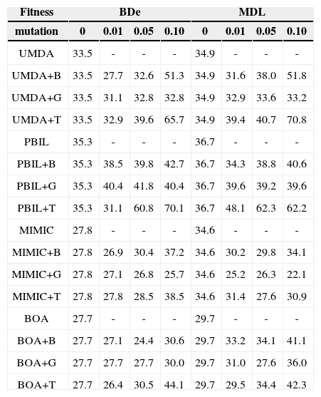
Comparison of precision (%) achieved by EDAs for the Asia data.
| Fitness | BDe | MDL | ||||||
|---|---|---|---|---|---|---|---|---|
| mutation | 0 | 0.01 | 0.05 | 0.10 | 0 | 0.01 | 0.05 | 0.10 |
| UMDA | 33.5 | - | - | - | 34.9 | - | - | - |
| UMDA+B | 33.5 | 27.7 | 32.6 | 51.3 | 34.9 | 31.6 | 38.0 | 51.8 |
| UMDA+G | 33.5 | 31.1 | 32.8 | 32.8 | 34.9 | 32.9 | 33.6 | 33.2 |
| UMDA+T | 33.5 | 32.9 | 39.6 | 65.7 | 34.9 | 39.4 | 40.7 | 70.8 |
| PBIL | 35.3 | - | - | - | 36.7 | - | - | - |
| PBIL+B | 35.3 | 38.5 | 39.8 | 42.7 | 36.7 | 34.3 | 38.8 | 40.6 |
| PBIL+G | 35.3 | 40.4 | 41.8 | 40.4 | 36.7 | 39.6 | 39.2 | 39.6 |
| PBIL+T | 35.3 | 31.1 | 60.8 | 70.1 | 36.7 | 48.1 | 62.3 | 62.2 |
| MIMIC | 27.8 | - | - | - | 34.6 | - | - | - |
| MIMIC+B | 27.8 | 26.9 | 30.4 | 37.2 | 34.6 | 30.2 | 29.8 | 34.1 |
| MIMIC+G | 27.8 | 27.1 | 26.8 | 25.7 | 34.6 | 25.2 | 26.3 | 22.1 |
| MIMIC+T | 27.8 | 27.8 | 28.5 | 38.5 | 34.6 | 31.4 | 27.6 | 30.9 |
| BOA | 27.7 | - | - | - | 29.7 | - | - | - |
| BOA+B | 27.7 | 27.1 | 24.4 | 30.6 | 29.7 | 33.2 | 34.1 | 41.1 |
| BOA+G | 27.7 | 27.7 | 27.7 | 30.0 | 29.7 | 31.0 | 27.6 | 36.0 |
| BOA+T | 27.7 | 26.4 | 30.5 | 44.1 | 29.7 | 29.5 | 34.4 | 42.3 |
For the Diabetes data set (Table 1), the bitwise and guided mutation-adopted EDAs showed better performance than their standard versions in terms of precision; the EDAs+B and EDAs+G with the best performance were around 10% more accurate than their typical counterparts. The transpose mutation-adopted EDAs showed markedly better performance than their counterparts, particularly those for UMDA+T and PBIL+T. In particular, PBIL+T (BDe, r=0.1) achieved 79.9% precision; however, the results for PBIL, PBIL+B, and PBIL+G were precisions of 42.0%, 46.6%, 50.8% respectively. Of the EDAs+T, MIMIC+T and BOA+T showed less improvement than UMDA+T and PBIL+T.
For the Asia data set (Table 2), EDAs+B and EDAs+G were not superior to their standard versions; PBIL+B and PBIL+G showed slightly improved performance. In contrast, the precisions of EDAs+T were superior to those of their standard versions; the best precisions were approximately 10%~35% higher than those of the standard versions. UMDA+T and PBIL+T showed better performance than UMDA/UMDA+B/UMDA+G and PBIL/PBIL+B/PBIL+G, giving best precisions of 70.8% and 70.1%, respectively. As compared to the other transpose versions, MIMIC+T exhibited less improvement in performance.
To make this study more informative, in Figs. 5, 6 and 7, we compare the changes in the proportion of arcs in the networks inferred by PBIL+T to investigate its superiority to its counterparts for the Asia data set (BDe, r=0.1). Fig. 5 shows the changes in the proportions of arcs correctly inferred by each algorithm. The proportion of arcs correctly inferred by PBIL+T increased rapidly with the number of generations; PBIL, PBIL+B, and PBIL+G were limited to inferring the correct arcs in the original network.


Fig. 6 shows the proportions of arcs in the reverse direction. PBIL+T also shows a rapid decrease compared to the other algorithms. Conversely, PBIL, PBIL+B, and PBIL+G exhibited substantially different behavior; the proportions of reverse arcs showed an increasing tendency as the generation increased.
Fig. 7 shows the proportions of additionally inferred arcs that are non-existent in the original network. In PBIL+T, the proportions of additional arcs drastically decrease as the number of generations increases, whereas PBIL, PBIL+B, and PBIL+G have difficulties in reducing the number of irrelevant additional arcs. The standard PBIL exhibited the most ineffective performance owing to premature convergence.
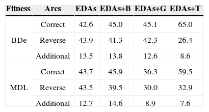
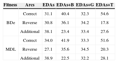
Tables 3 and 4 list the comparison results of the average proportions of arcs in the network learned by EDAs, EDAs+B, EDAs+G, and EDAs+T, for the Diabetes and Asia data, respectively. From the table, we see that EDAs+T are superior to EDAs, EDAs+B, and EDAs+G; for inferring the correct arcs, EDAs+T were about 10%~23% more accurate than the conventional methods. The present evaluation has verified the potential utility of the transpose mutation-adopted EDAs.
The results of the comparison calculations indicate that the transpose mutation gave the greatest enhancement of learning performance for the PBIL+T algorithm. PBIL+T uses a learning rate a to control the ratio of recently sampled individuals to individuals of the previous generation in order to obtain the new probability model; there is no general agreement on the value to use for the optimal choice of a. In this study, we empirically tested various a values and reported their influence on the learning results. Fig. 8 shows the precision of PBIL+T for a=0.1, 0.3, 0.5, 0.7, and 0.9, for the Asia data (with d=50 fixed). Of the a values considered, PBIL+T gave the best precisions at a=0.7; it provided more stable performance than the other choices at r=0.1, 0.15, and 0.2. PBIL+T with a=0.1 showed the most ineffective performance over the different mutation rates.

In addition, we investigated the influence of the choice of a for different population sizes, as shown in Fig. 9 (with r=0.15 fixed). PBIL+T with a=0.7, 0.9 showed the best result at d=50. Stable performance was obtained at a=0.9, whereas PBIL+T with a=0.1 gave lower precisions than with other a values. Moreover, we assessed the difference in performance using a statistical test. The paired t-test at 0.05 significance level revealed that for the Asia and Diabetes data sets, PBIL+T is significantly superior to its counterparts for almost all the cases. Thus, these results highlight the effectiveness of the proposed PBIL+T method.
5Conclusion
It was well established that the incorporation of mutation into EDAs increases the diversity of genetic information in the population, thereby avoiding premature convergence into a suboptimal solution. As compared to the corresponding EDAs, the transpose mutation-adopted EDAs are superior and effective algorithms for learning Bayesian networks. Of the transpose versions tested, PBIL+T was shown to be the best option in most cases; it is the most suitable option when no prior knowledge on the properties of the data is available. Besides the issues mentioned in the present study, several issues require further investigation. Although PBIL+T is considered the most powerful algorithm in Bayesian structure learning, further investigation is required to compare the performance of transpose mutation in various EDAs for other problems. Such analysis would be complicated by the fact that the choice of EDAs and mutation is a data-dependent task. Thus, future studies should focus on the development of a method for automatically selecting the most appropriate EDAs and mutation according to the characteristics of the data set.
This research was supported by Kyungpook National University Research Grant of KNU Convergence Program, 2011.