


The problem concerning the nature and the function of the dead space is of basic importance for the full comprehension of the respiratory physiology and pathophysiology. To study the effect of an imposed external dead space on the optimal respiratory control system, we simulated the optimal neuro-muscular drive and respiratory signals, including instantaneous airflow and lung volume profiles, with dead space loading under hypercapnia. The dead space measurement model by Gray was employed and the human respiratory control simulator based on an optimality hypothesis was implemented. The ventilatory control simulations were performed with external dead space loading of 0, 0.4 and 0.8 liters under rest condition (PICO2=0%) and CO2 inhalation of 3% to 7%. The optimization of the respiratory signals and model behavior of the optimal respiratory control under dead space loading and hypercapnia were verified and found to be in general agreement with experimental findings.
Extended studies on the concept of dead space have been made in the last half-century. The problem concerning the nature and the function of dead space is of basic importance for the full comprehension of the respiratory physiology and pathophysiology [1-6]. Bohr used a mass balance method to measure dead space through the information of tidal volume, mixed alveolar gas, and expired alveolar gas compositions. Klocke [7] acknowledged that dead space values were important in the past, because alveolar ventilation was calculated from total ventilation using an assumed or empirical value for dead space. Fowler [8] determined dead space volume using Bohr’s formula, with the conclusion that the regional non-uniformity of ventilation and lung volume were the most important factors in determining the dead space volume. Pappenheimer [9] proposed a new technique that utilizes constant alveolar gas tensions for measuring VD, PACO2 and PACO2, which provides a graphic solution of the Bohr formula. Although it appeared a better method than Coon [10], Wolff [11] have described latter because of its independence of metabolic rate, however, the method depended on constancy of VD. Maruyama [12] studied ventilatory response during external dead space breathing and CO2 inhalation for given increase in PETCO2 with different levels of PETO2 (hyperoxia, normoxia, and hypoxia) in human. Lofaso [13] investigated the effect of positive or negative inspiratory pressure on respiration under external dead space loading. Poon [14] examined the effects of airway CO2 loading on the response of ventilation-CO2 output during exercise with and without external dead space.
The optimization and simulation techniques and tools have been well developed during the past decades and been widely applied in the field of engineering design [15,16] and biomedical research [17-20]. An earlier research by Poon [21] suggested that the ventilatory responses to CO2 inhalation and exercise and can be predicted by the minimum criteria of a controller objective function including chemical and mechanical costs of breathing. It was later extended to model the integrative control of V˙E and respiratory pattern, by expressing the breathing work rate in terms of the respiratory neural drive P(t) [22]. The simulator implemented by Lin [17] constructed was based on the optimal respiratory control model with LabVIEW. Subject to any change in ventilation, we may observe the respiratory response and monitor the effect of the imposed experiments on wave shapes to various chemical stimuli in real-time.
An earlier study [18] was aimed to simulate and compare the effect of external dead space (EDS) loading on the ventilatory response of two distinct dead space measurement models, derived from Gray and Coon. Predicted behaviors with corresponding ventilatory responses were investigated and compared with experimental findings. While both dead space models produced satisfactory predictions on optimized V˙Evs.PCO2, V˙Avs.PCO2, F vs. PICO2, VT vs. PICO2, VD-total vs. VT, VD-total/VT vs. VT, V˙Evs.VT and V˙Avs.VT relationships, Gray’s model provided better correlation and more consistent results throughout most of the ventilatory responses.
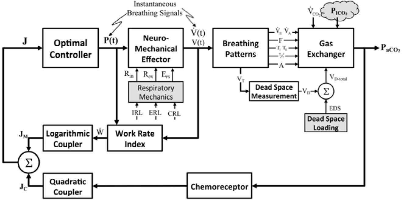
2MethodPrevious researches [17,18] have successfully proposed and implemented a simulation strategy based upon a mathematical model of the optimal respiratory control with MATLAB and LabVIEW. In current study, simulations were based upon the mathematical modeling of the optimal respiratory control, as illustrated in Fig. 1, with LabVIEW platform. The controller of the optimal chemical-mechanical respiratory control model of Fig. 1 is driven by both chemical and neuro-mechanical feedback signals. Figure 1 shows the coupling of chemical cost and mechanical cost. The fundamental hypothesis of the model is that a total cost function can be formulated to reflect the balance of a combined challenge (J) due to the chemical (JC) and mechanical cost (JM) of breathing [10]. The respiratory control feedback system is modeled with four major functional blocks: the plant, the feedback path, the controller, and the effector. The mathematical descriptions of four functional blocks have been detailed in earlier researches [17] and are outlined briefly below:
![The mathematical modelling of the optimal chemical-mechanical respiratory control [17].](https://static.elsevier.es/multimedia/16656423/0000001200000006/v2_201505081706/S166564231471661X/v2_201505081706/en/main.assets/gr1.jpeg?xkr=ue/ImdikoIMrsJoerZ+w997EogCnBdOOD93cPFbanNcX6PcOHo8VDqRKrp6xHZ/NlPxKUvo805ICrHlplwxcm7hYIESfjCCTNDlVokL+8rN3BbokVvmcPjARh27za9sJ5qQejMOkdJE5m+uzI0VibngclXqq48RJIAsJGlcBVYBNGWSToMGm66Y+Iu2HV4OthgQ5g3LzGg72WZpxQ6xOjFXKfLy/8ZWOFM92xICDZaFN2sO97nchZ2dffSCHGx9AWJFhr7F22pBthG7Xli+rLKbuyXp6IRs49TdDX3pyGF8veGmLSPABYsaD7mRdMWcZrZY+2G6bD/OUqnbPWfIE6Q== "The mathematical modelling of the optimal chemical-mechanical respiratory control [17].")
The mathematical modelling of the optimal chemical-mechanical respiratory control [17].
The plant describes the events of the pulmonary exchange subject to the control signal V˙E(total ventilation in one minute, l/min) and disturbances in the inhaled and metabolic CO2 and O2 (PICO2/PIO2, Torr, V˙CO2/V˙O2, l/min), and lactic acidosis. The system’s outputs are the pressures of arterial CO2 and O2 (PaCO2/ PaO2, Torr), and [H+]a (arterial H-ion concentration, mole/l). Because the conditions of normoxia and normal acid base condition will be assumed in the paper, only the effects on PaCO2 will be considered. The gas exchanger equation describes the dependence of the arterial blood gas tension on the total ventilation and other disturbances are given as [10,11,13]:
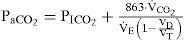
where PaCO2 is assumed to be identical to mean alveolar PCO2. Equation (1) describes the steady-state effect of ventilation on PaCO2 subject to any disturbances in the inhaled and metabolic production of CO2.
ChemoreceptorsAs depicted in Fig. 1, the feedback loop consists of two chemosensory structures, known as the central and peripheral chemoreceptors. The total chemical stimulation level of the controller (IO, impulses/sec), the sum of the central (IC, impulses/sec) and peripheral chemoreceptor stimulus (IP, impulses/sec), can be expressed as a linear function of PaCO2 [17,23].
Neuro-Mechanical EffectorInstantaneous airflow is known to be controlled physiologically by neural impulses from the respiratory center (controller). The neuro-mechanical effector, which relates the neural respiratory output to the resultant mechanical airflow, is required for optimizing the neural input to the respiratory muscles to optimize the ventilatory airflow (V˙(t), L/min). The mechanical work of respiration results from the frictional resistance to airflow in the airways and the stretching of the elastic walls of the lungs and thorax. The neuro-mechanical effector can be described by the electrical analog of the linear or nonlinear model of respiratory mechanics, which characterizes the resistance of the airways, the lung inertance, and the compliance of the alveoli. To simplify the mechanical model of the respiratory system, the inertance was neglected when switching from the R-L-C model to the R-C model. In previous studies [17,18,21,22], we described the neuro-mechanical effector by using the electrical R-C model (Fig. 3(A)), based on a lumped-parameter model proposed by Younes and Riddle [24], for relating respiratory neural and mechanical outputs. In this model, the equation of motion is given by the following dynamic equation:
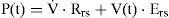
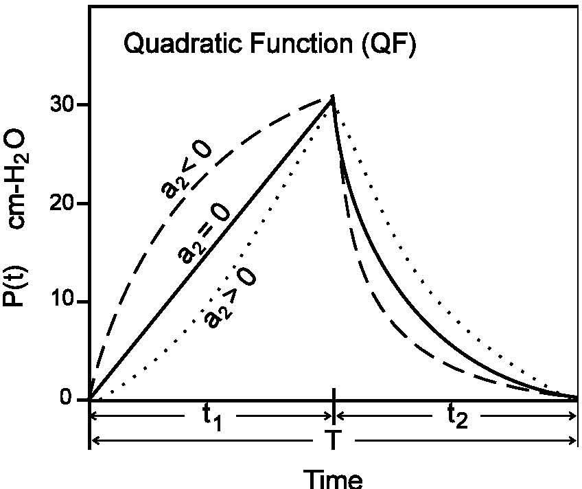
The parameters Rrs (cm-H2O.l-1.sec) and Ers (=1/Crs, cm-H2O/I) represent the total flow-resistive and volume-elastic components, respectively, which include the passive resistances and elastance of the lung, chest wall, and airways. The waveshape of the neuro-muscular drive (P(t), cm-H2O) is modeled into an inspiratory and expiratory phase. The inspiratory drive is approximated by a quadratic function and the expiratory pressure is represented by an exponential discharge function of the form (Fig. 2) [18,22]:


where the parameters a0 and a1 in Eq. (3) represent the net driving pressure and its rate of rise at the onset of the neural inspiratory phase, and the parameter a2 describes the shape of the wave; t1 (sec) and t2 (sec) represent the neural inspiratory and expiratory duration, respectively. In Eq. (4), P(t1) is the peak inspiratory pressure (cm-H2O) and τ denotes the rate of decline of inspiratory activity.
Optimal ControllerPoon [21,22] proposed and Lin [17,18] verified that an optimal controller might counterbalance the metabolic needs versus energetic needs of the body, and the resulting compromise would determine the ventilatory response. Rather than a reflex response to the chemical stimulus, the fundamental hypothesis of the optimal controller is that a total cost function (J) can be formulated to reflect the balance of a combined challenge due to chemical (JC) and mechanical (JM) cost of breathing [17,21,22]. The optimal control output is determined by the minimum of J, which consists of the square law for chemical feedback and logarithmic law for mechanical feedback, conforming to Steven’s law and Weber-Fechner law of sensory reception, respectively. On the other hand, the respiratory work rate W˙, is assumed to be an explicit function of the respiratory neural drive and can be parameterized by the mechanical constraints of the respiratory system although this takes a quantitative description of the mechanical effector system.
Work Rate Index. Several mechanical indices have been previously studied for respiratory optimization [17, 21]. In the implemented simulator of current study, the mechanical work rate of inspiration and expiration are evaluated to predict the inspiratory waveshape and ventilatory responses to various types of system inputs.
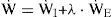
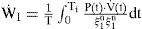
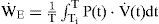
In Eq. (5), the total mechanical index is assumed to be a weighted sum of the inspiratory and expiratory indexes with a weighting parameter λ, and W˙,W˙I, and W˙E represent the total respiratory, inspiratory, and expiratory work rate (kg-m/sec), respectively [17]. The efficiency factors ξ1 and ξ2 of Eq. (7) account for the effects of the respiratory-mechanical limitation and the reduction in the neuro-mechanical efficiency with increasing effort. The overall efficiency is dependent on two factors: the maximal (Pmax) and the maximum rising rate of neuro-muscular drive (P˙max).
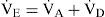
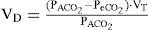
Dead Space ModelingWhen V˙A was defined as the miniute volume of gas that, when in CO2 equilibrium with arterial blood, must be expired to maintain V˙CO2. Thus V˙A is equal to the minute volume of gas expired from alveolar structures only when all these structures have a mean PaCO2 value equal to PaCO2. Defining V˙A in terms of V˙CO2, then dead-space ventilation (V˙D) is defined as [25].
The Eq. (8) can further be developed, firstly by Bohr, to measure the physiological dead space.
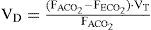
where FACO2 is alveolar CO2, FECO2 is the fractional concentration of CO2 from mixed expired gases.
The Bohr equation is considered to be complicated since it is based upon the fact that all CO2 comes from alveolar gas and the exhalation of CO2 can therefore be used to measure gas exchange or lack of gas exchange if there is alveolar dead space. For each tidal volume there will be a proportion of dead space (anatomical) but the amount of gas that is left over should take part in gas exchange.
Gray [25] proposed a dead space formulation that included the Bohr Formula, Washout equation and Virtual dead space equation. One of the original uses of the Bohr formula was to calculate alveolar composition from knowledge of the anatomical dead space and thus obviate the difficulties of alveolar sampling. Unfortunately the formula uses a “dead air” variable and not a space at all. Experiments also demonstrated the dependence of expired dead air volume on the tidal volume, particularly for the lower tidal volumes. In respiratory physiology the Bohr formula is applied to find many significant results. The washout equation is useful because in the washout phenomenon, the volume of the expired dead air must be a function of the expired tidal volume.
As a consequence of the washout phenomenon, the volume of expired dead air must be a function of the expired tidal volume. Rohrer suggested approximating this relationship by the physical law for the washing out of a rigid uniform cylinder by uniform laminar airflow.
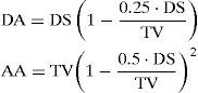
where DA represents the virtual dead air, AA represents virtual alveolar air, TV represents the volume of expiration flow, and DS represents the fixed volume of the cylinder. By rearrangement of the washout equation of Eq. (11) and combining it with the Bohr formula, Gray [25] obtained:
where FI and FE are the composition of inspired and expired air, respectively, and F¯A is the mean composition of the altered components in the virtual alveolar air.
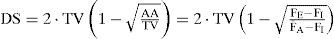
Various reasons were given by Gray [25] for expecting the virtual dead space to increase with the inspiratory tidal volume. Gray firstly assumed that the virtual dead space could be approximated by a simple linear function [25]:

where VDS0 is the standard virtual dead space at zero tidal volume, KDS is the increment in virtual dead space per unit increment in tidal volume. The empirical constants were obtained from experiments on five medical students by statistical fitting of the experimental data and permit evaluation of the fundamental variables VDS0 and KDS. Based on the experimental results, the two dead space properties were effectively reduced by approximating KDS as equal to 18 of VDS0, thus reducing Eq. (13) to
To account for the changes in anatomic dead space with airway caliber, Eq. (14) was employed with following empirical relation suggested [26]:
where VC is vital capacity which ranging between 3 and 5 liters for normal adults.
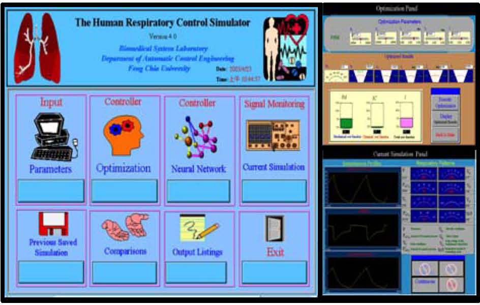
3Simulation Results and DiscussionThe simulator’s human-machine interface was constructed with a multilayered structure from main panel for an expandable modular design using the LabVIEW platform. Figure 3 shows the human respiratory control simulator’s main control panel. From the main panel of Fig. 3, the user can initiate a simulation via the input panel by entering respiratory parameters including V˙CO2 (metabolic rate of CO2), PICO2 (partial pressure of inhaled CO2), Rin (inspiratory airway resistance), Rex (expiratory airway resistance), Ers (lung elastance), and EDS (external dead space loading).
![Main panel (left), optimization panel (upper right), and signal monitoring window for current simulation (lower right) in the simulator [17].](https://static.elsevier.es/multimedia/16656423/0000001200000006/v2_201505081706/S166564231471661X/v2_201505081706/en/main.assets/gr3.jpeg?xkr=ue/ImdikoIMrsJoerZ+w997EogCnBdOOD93cPFbanNcX6PcOHo8VDqRKrp6xHZ/NlPxKUvo805ICrHlplwxcm7hYIESfjCCTNDlVokL+8rN3BbokVvmcPjARh27za9sJ5qQejMOkdJE5m+uzI0VibngclXqq48RJIAsJGlcBVYBNGWSToMGm66Y+Iu2HV4OthgQ5g3LzGg72WZpxQ6xOjFXKfLy/8ZWOFM92xICDZaFN2sO97nchZ2dffSCHGx9AWJFhr7F22pBthG7Xli+rLKbuyXp6IRs49TdDX3pyGF8veGmLSPABYsaD7mRdMWcZrZY+2G6bD/OUqnbPWfIE6Q== "Main panel (left), optimization panel (upper right), and signal monitoring window for current simulation (lower right) in the simulator [17].")
Main panel (left), optimization panel (upper right), and signal monitoring window for current simulation (lower right) in the simulator [17].
User selects controller from alternatives, optimization to optimize the respiratory waveforms and breathing pattern, or neural network to use both the back-propagation neural network and forward model to obtain simulated results without going through the time-consuming optimization process. Selecting the optimization control opens the window shown on the upper right of Fig. 3. In the upper part of the window, the user is requested to define the initial parameters essential to the optimization. Once all of the initial estimates are entered, the user selects the “Execute Optimization” control. The optimization runs until the numerical calculation is completed and an optimum is reached. Clicking the “Display optimized results” control displays the optimized variables a0, a1, a2, t1, t2, and τ in the center of the window. The obtained optimized parameters can then be used to compose the isometric pressure profile with Eq. (3) and Eq. (4). The simulation results can be observed through the signal monitoring of current simulation panel, as shown in the lower right of Fig. 3. The “Instantaneous Profiles” windows demonstrate three respiratory waveforms to be monitored: neuromuscular driving Pressure P(t), airflow V˙(t) and lung volume V(t). The respiratory patterns, including f, PaCO2, VT, PaO2, V˙CO2,V˙O2, VO, TI, TE, and TI/T, are shown through the use of virtual instruments of LabVIEW and located in the upper right of the panel.
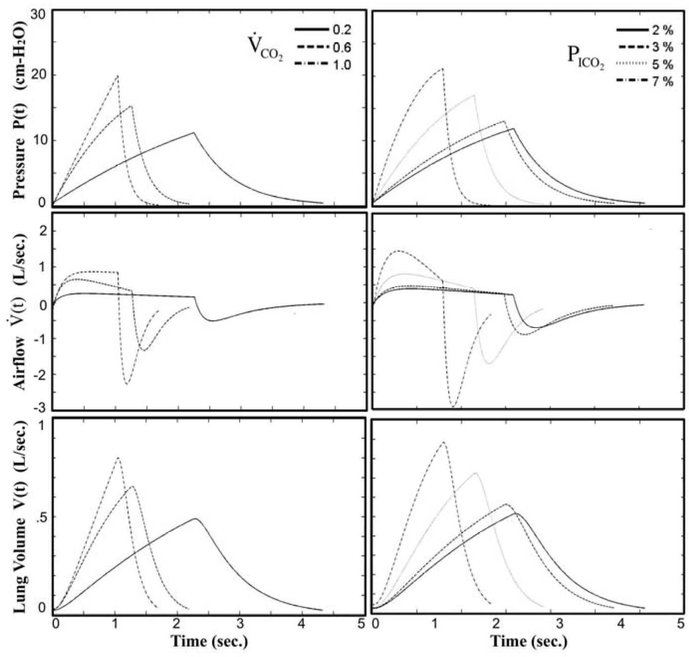
The resultant waveforms were simulated and monitored at varying levels of CO2 inhalation and exercise in earlier study [17] without external dead space loading. As shown in Fig. 4, the instantaneous neuro-muscular driving pressure P(t), airflow rate V˙(t), and volume V(t), from top to bottom, respectively, are summarized at various levels of exercise CO2 output (V˙CO2 = 0.2, 0.6, 1.0) and inhaled CO2 (PICO2=2%, 3%, 5%, 7%). The simulator is built to be a useful platform as the model behavior of respiratory control can be investigated by examining the instantaneous responses of the waveforms under various breathing situations.
, top), airflow rate (V˙(t) middle), and lung volume (V(t), bottom) over a complete breathing cycle at various levels of exercise CO2 output (left) and inhaled CO2 (right) without external dead space loading.")
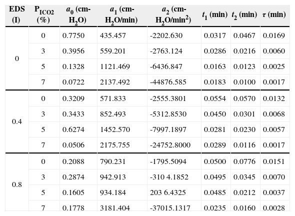
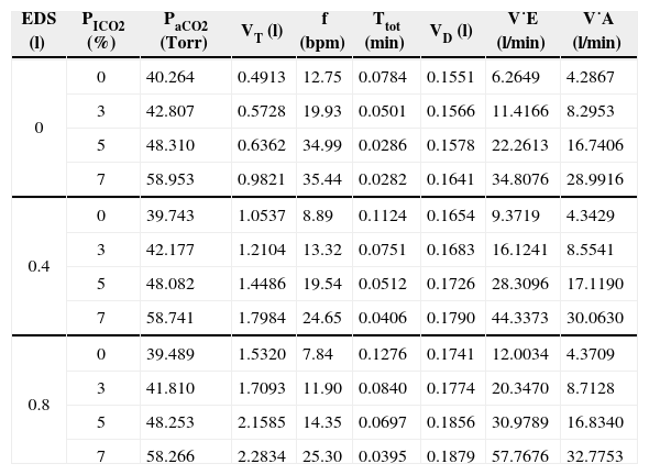
The results of current study were tabulated in Table 1 and Table 2. In Table 1, the optimized results of the optimization variables a0, a1, a2, t1, t2, and τ under simulated EDS and PICO2 levels were presented. By applying the Eqs. (3) and (4) with the optimized results of Table 1, the optimized neuro-muscular driving pressure profiles can be figured in the form of Fig. 4. On the other hand, with the use of the dynamic equation of Eq. (2) and proper mathematical operations [17,22], the optimized instantaneous airflow and lung volume profiles can also be derived. The tidal volume was obtained from lung volume profile (VT=V(t1)-V(t1+t2)), and all the resultant breathing patterns, including PaCO2, f, TTOT, VD, V˙E, and V˙A, were consequently derived as revealed in Table 2.
Results of the optimized parameters for neuro-muscular drive under added EDS and CO2 inhalation.
| EDS (I) | PICO2 (%) | a0 (cm-H2O) | a1 (cm-H2O/min) | a2 (cm-H2O/min2) | t1 (min) | t2 (min) | τ (min) |
|---|---|---|---|---|---|---|---|
| 0 | 0 | 0.7750 | 435.457 | -2202.630 | 0.0317 | 0.0467 | 0.0169 |
| 3 | 0.3956 | 559.201 | -2763.124 | 0.0286 | 0.0216 | 0.0060 | |
| 5 | 0.1328 | 1121.469 | -6436.847 | 0.0163 | 0.0123 | 0.0025 | |
| 7 | 0.0722 | 2137.492 | -44876.585 | 0.0183 | 0.0100 | 0.0017 | |
| 0.4 | 0 | 0.3209 | 571.833 | -2555.3801 | 0.0554 | 0.0570 | 0.0132 |
| 3 | 0.3433 | 852.493 | -5312.8530 | 0.0450 | 0.0301 | 0.0068 | |
| 5 | 0.6274 | 1452.570 | -7997.1897 | 0.0281 | 0.0230 | 0.0057 | |
| 7 | 0.0506 | 2175.755 | -24752.8000 | 0.0289 | 0.0116 | 0.0017 | |
| 0.8 | 0 | 0.2088 | 790.231 | -1795.5094 | 0.0500 | 0.0776 | 0.0151 |
| 3 | 0.2874 | 942.913 | -310 4.1852 | 0.0495 | 0.0345 | 0.0070 | |
| 5 | 0.1605 | 934.184 | 203 6.4325 | 0.0485 | 0.0212 | 0.0037 | |
| 7 | 0.1778 | 3181.404 | -37015.1317 | 0.0235 | 0.0160 | 0.0028 |
Results of the optimized breathing patterns under added EDS and CO2 inhalation.
| EDS (l) | PICO2 (%) | PaCO2 (Torr) | VT (l) | f (bpm) | Ttot (min) | VD (l) | V˙E (l/min) | V˙A (l/min) |
|---|---|---|---|---|---|---|---|---|
| 0 | 0 | 40.264 | 0.4913 | 12.75 | 0.0784 | 0.1551 | 6.2649 | 4.2867 |
| 3 | 42.807 | 0.5728 | 19.93 | 0.0501 | 0.1566 | 11.4166 | 8.2953 | |
| 5 | 48.310 | 0.6362 | 34.99 | 0.0286 | 0.1578 | 22.2613 | 16.7406 | |
| 7 | 58.953 | 0.9821 | 35.44 | 0.0282 | 0.1641 | 34.8076 | 28.9916 | |
| 0.4 | 0 | 39.743 | 1.0537 | 8.89 | 0.1124 | 0.1654 | 9.3719 | 4.3429 |
| 3 | 42.177 | 1.2104 | 13.32 | 0.0751 | 0.1683 | 16.1241 | 8.5541 | |
| 5 | 48.082 | 1.4486 | 19.54 | 0.0512 | 0.1726 | 28.3096 | 17.1190 | |
| 7 | 58.741 | 1.7984 | 24.65 | 0.0406 | 0.1790 | 44.3373 | 30.0630 | |
| 0.8 | 0 | 39.489 | 1.5320 | 7.84 | 0.1276 | 0.1741 | 12.0034 | 4.3709 |
| 3 | 41.810 | 1.7093 | 11.90 | 0.0840 | 0.1774 | 20.3470 | 8.7128 | |
| 5 | 48.253 | 2.1585 | 14.35 | 0.0697 | 0.1856 | 30.9789 | 16.8340 | |
| 7 | 58.266 | 2.2834 | 25.30 | 0.0395 | 0.1879 | 57.7676 | 32.7753 |
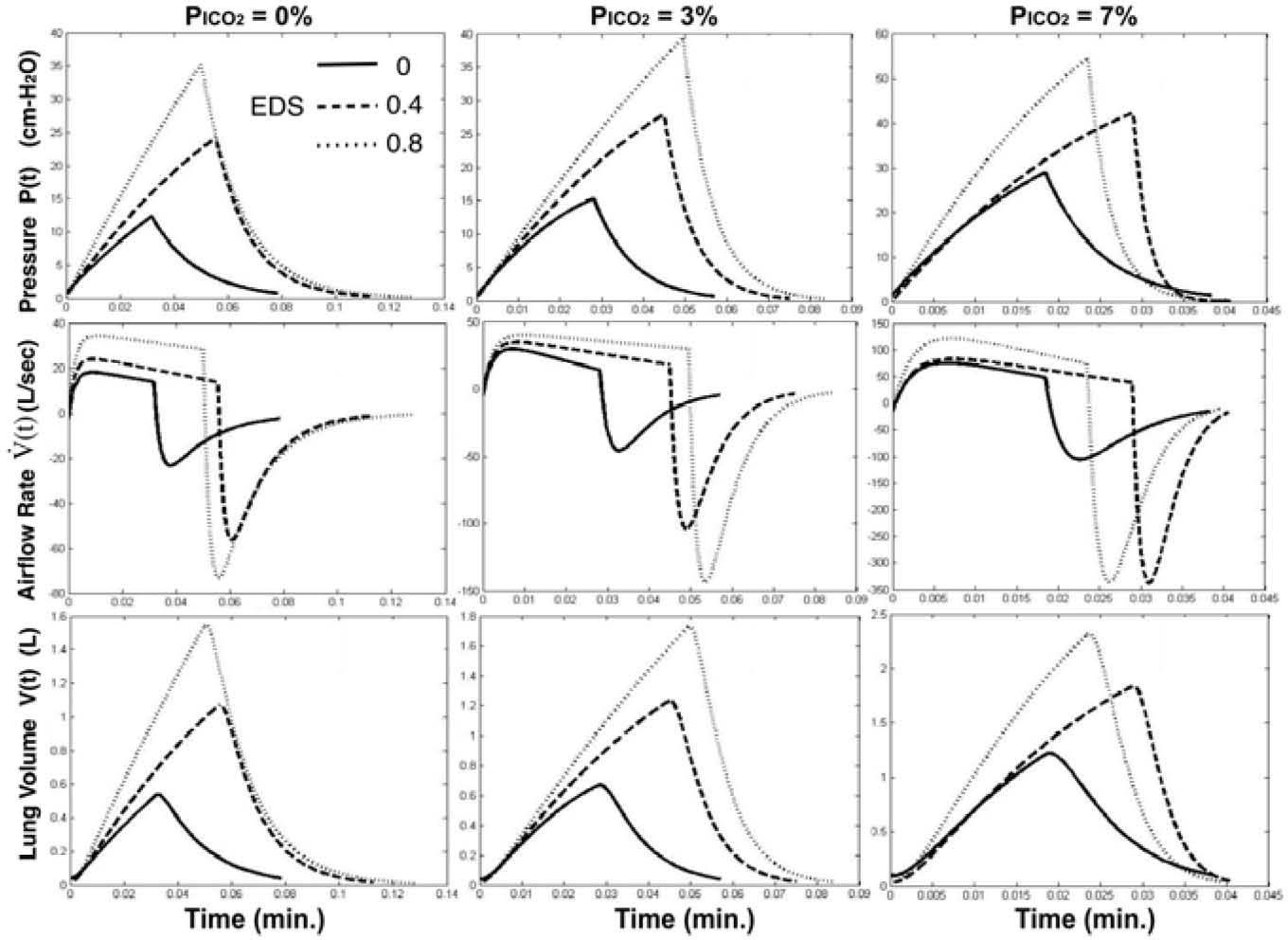
To examine the effect of an imposed dead space loading on the optimized instantaneous respiratory waveforms under different levels of CO2 inhalation, Fig. 5 depicts the profiles with EDS=0, 0.4, and 0.8 l. As an EDS of 0.4 (l) was imposed and PICO2=0% (left column of Fig. 5), in comparison with EDS=0, the optimized neuro-muscular drive P(t) (top row of Fig. 5) attains a higher amplitude with prolonged inspiratory duration (t1) and higher duty cycle (TI/T). As PICO2 was increased to 3% (middle column of Fig. 5) and 7% (right column of Fig. 5), the change of the waveshapes in P(t) displayed little difference with that of 0% but with higher magnitude. However, as an EDS of 0.8 (l) was imposed, we found that inspiratory duration and duty cycle were reduced to be less than those of EDS=0.4 (I) under the cases of PICO2=0% and 7%.
 on optimized waveshapes of P(t) (top), V˙(t) (middle), and V(t) (bottom) under PICO2= 0% (left), 3% (middle), and 7% (right).")
The airflow profiles (middle row of Fig. 5) do not show substantial change in shape although the peak inspiratory and expiratory flow achieved higher rates with increased EDS loading or higher CO2 inhalation level. The lung volume profiles also appear insignificant difference in shape but higher peak volumes with increased EDS
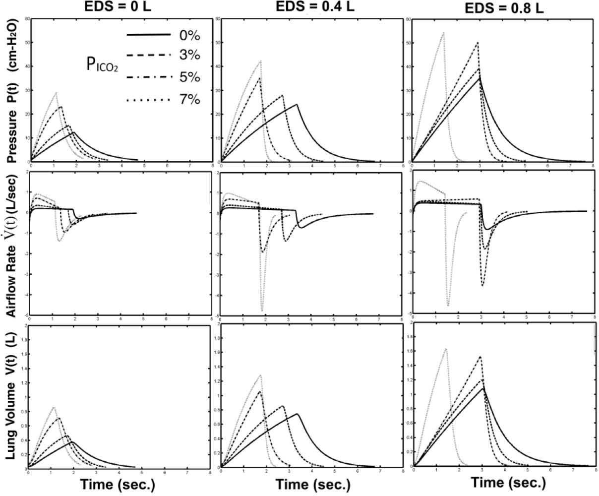
Figure 6 shows the effect of increased concentration of CO2 inhalation on the optimized respiratory waveforms under three imposed EDS loading levels (EDS=0, 0.4, and 0.8 l). Without dead space loading (EDS=0), the waveforms of P(t) (top row of Fig. 5) are shaped as higher in rising rate (larger in a1) and more concave upward (more negative in a2) with increased PICO2. The effect of increase PICO2 on inspiratory duration and duty cycle is not as significant as on the increasing breathing frequency (decreasing period). As the imposed EDS was increased to 0.4 (middle column of Fig. 6) and 0.8 liters (right column of Fig. 6), the rising rates in P(t) become steeper as the concavities of the waveshape seem lesser. On the other hand, based on the airflow profiles on Fig. 6 (middle row), we also find that the increased PICO2 level had shaped the V˙(t) from a rectangular-like waveform to a decending-like waveform with higher inspiratory and expiratory peak flows. As the EDS were increased to either 0.4 or 0.8 liters, the increasing in peak flow rate and the waveshaping in the inspiratory phase became more significant.
 on waveshapes of P(t) (top), V˙(t) (middle), and V(t) (bottom) under EDS= 0 (left), 0.4 (middle), and 0.8 liters (right).")
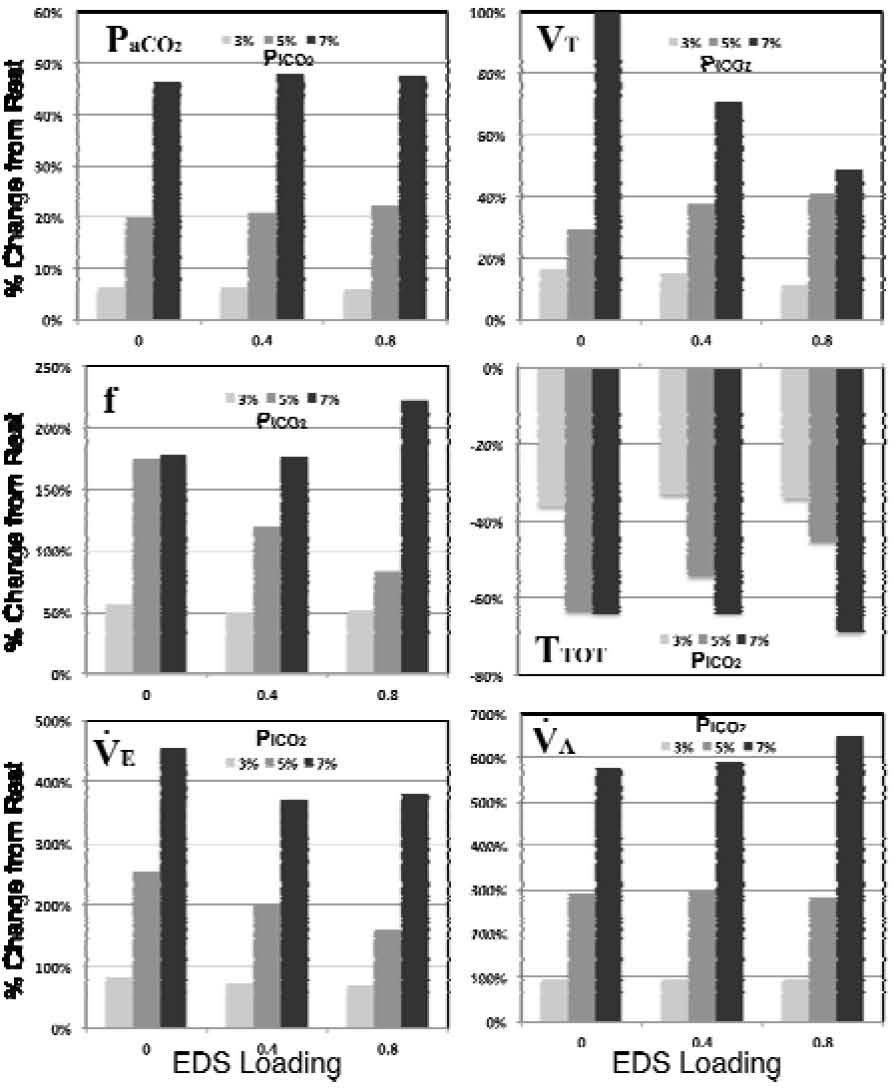
In Fig. 7, the effect of EDS loading (EDS=0, 0.4, and 0.8 l) on the optimized breathing patterns under various levels of CO2 inhalation (PICO2=3%, 5%, and 7%), which were depicted in Table 2, are further summarized based on their percentage changes from rest condition (PICO2=0%). The hypercapnic response in PICO2 (upper left of Fig. 7) seems to be unaffected among three levels of EDS loadings. At PICO2=3%, the increased EDS loading appears to have little effect on the variation in tidal volume (VT, upper right of Fig. 7). However, the changes in VT slightly increased (form 29.49% to 40.89%) at PICO2=5%, and significantly decreased (from 99.9% to 49.05%) at PICO2=7%, with elevated level of EDS loadings. The ventilatory response on tidal volume (VT) should always be considered together with breathing frequency (f) for the attained total ventilation level (V˙E=VT×f) under any chemical or exercise stimuli. An opposite effect to the variation in tidal volume can be observed in breathing frequency as EDS loading was imposed during CO2 inhalation, as was depicted in middle left of Fig. 7. Under different level of EDS, the changes in f are found to be nearly the same (≅50%) at PICO2=3%, and display a significant decreasing (from 174.43% to 83.04%) and slight increasing (from 177.96% to 222.70%) at PICO2=5% and 7%, respectively. As a result, we attain a minute ventilation level at marginally decreasing fashion with increasing EDS loading under each PICO2 level, as was depicted in lower left of Fig. 7. Meanwhile, the resultant variations in alveolar ventilation V˙A(lower right of Fig. 7) are considerably stable in comparisons with the other breathing patterns at each CO2 inhalation level.
4Conclusions with EDS loading at 0, 0.4, and 0.8 (l) under different levels of CO2 inhalation (PICO2= 3%, 5%, 7%). Left (from top to bottom): PICO2, f, and V˙E; Right(from top to bottom): VT, TTOT, and V˙A.")
With the use of the optimal respiratory control, a unified prediction of exercise and chemical responses was shown entirely in terms of conventional feedback-mechanisms instead of a separate stimulus signal, which has never been clearly demonstrated. With this model, a human respiratory control simulator is constructed to simulate the ventilatory responses under muscular exercise and CO2 inhalation. We have examined the effects of external dead space loadings on the resultant ventilatory responses, including V˙A-PaCO2,V˙E-V˙CO2,V˙A-V˙CO2,F-V˙CO2,VT-V˙CO2, and VT-PaCO2 relationship, in earlier studies [17] for the simulations with different levels of EDS. Current study is aimed to explore the effect of the imposed dead space loading on the optimized respiratory profiles of pressure, airflow, and lung volume under increased levels of CO2 inhalation. The simulation results show that higher amplitude with prolonged inspiratory duration and higher duty cycle were attained as EDS=0.4 (l) was imposed. The increase of EDS =0.8 (l) showed opposite effects on the inspiratory duration and duty cycle under PICO2=0% and 7%. No significant change in the waveshapes of these respiratory profiles was found with the imposed dead space loading under CO2 inhalation. Current study attained valuable results in simulations of imposed dead space on respiratory control with the optimal respiratory control model. Further work can be extended to include the effects of respiratory mechanical (resistive or elastic) loading along with EDS loading.
This study was supported by grants NSC 101-2221-E-035-005 from the National Science Council, Taiwan.