


Researchers put efforts to discover more efficient ways to classification problems for a period of time. Recent years, the support vector machine (SVM) becomes a well-popular intelligence algorithm developed for dealing this kind of problem. In this paper, we used the core idea of multi-objective optimization to transform SVM into a new form. This form of SVM could help to solve the situation: in tradition, SVM is usually a single optimization equation, and parameters for this algorithm can only be determined by user’s experience, such as penalty parameter. Therefore, our algorithm is developed to help user prevent from suffering to use this algorithm in the above condition. We use multi-objective Particle Swarm Optimization algorithm in our research and successfully proved that user do not need to use trial – and – error method to determine penalty parameter C. Finally, we apply it to NIST-4 database to assess our proposed algorithm feasibility, and the experiment results shows our method can have great results as we expect.
Pattern recognition has been a frequently encountered problem with a wide range of application such as fingerprint, face, voice and so on. The problem can be summarized to a decision-making process to distinguish if the test sample is complied with the criteria made by the database. Generally, the classification problem can be categorized as binary classification problems (two-class classification) and multiclass classification problems [1]. Nowadays, binary classification problem can be solved by many algorithms. For instance, neutral networks, Naïve Bayes classifier, C4.5 decision tree, and also support vector machine (SVM). Algorithms mentioned above can be available in multiclass problems.
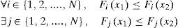
Multi-objective optimization idea was aroused recent years [2]. This kind of algorithms is developed on a core idea of Pareto frontier. Before this idea was known for people, we can only handle our optimization problem as a single objective problem as following:
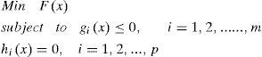
where x is called decision variables, F(x) is objective function, and gi(x) and hi(x) are inequalities and equalities constraints. Note that m and p is the number constraints.
However, in realistic application, we often have at least two or more objectives which are not only interacting but probably conflicting. Generally, a multi-objective optimization problem can be expressed as:
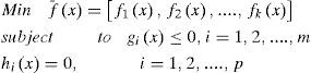
The desired solution for multi-objective problems is in the form of “trade-off or compromise among the parameters that would optimize the given objectives. The optimal trade-off solutions among objectives constitute the Pareto front.
In this paper, we proposed an evolutionary algorithm to reform the traditional SVM algorithm from a single objective optimization problem to a multi-objective optimization problem. The results show that we succeed to get a feasible solution without knowing penalty coefficient C and this algorithm is employed to classify fingerprint classification.
2Optimization algorithm and support vector machineThis section presents the essential theory in this paper. The definition, operations, and algorithms for multi-objective optimization algorithm and SVM are introduced in Sec 2.1, Sec2.2 and Sec 2.3 then presents the idea of our proposed algorithm.
2.1Multi-objective OptimizationThe definition of this problem can be seen from (1). Multi-objective optimization (MOO) deals with generating the Pareto frontier which is the set of non-dominated solutions for problems having more than one objective. The following definitions are shown in [15].
Definition 1Assume there are two solutions x1 and
x2, if both of them are complied with the following rule, we said x1 dominates x2.
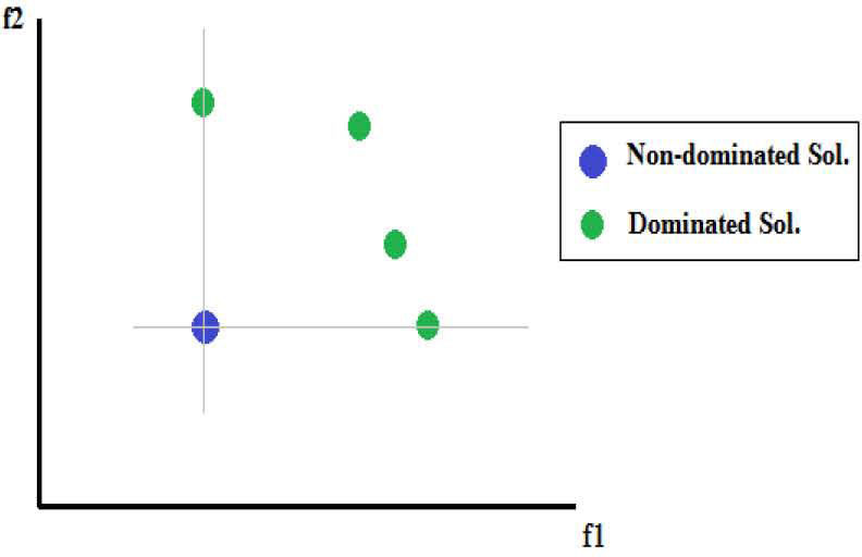
x1 is non-dominated solution, while x2 is so-called dominated solution. The relation is shown in Figure 1.

Figure 1 is shows the relation of dominated and non-dominated sets. In this figure, f1 and f2 are values for the two objective functions. This example figure is a model that both f1 and f2 functions are required to be minimized. The dominated solution is the green points (i.e., x2) and the non-dominated solution is the blue points (i.e., x1). With definition 1, it is shown that f1 and f2 for the non-dominated solution are either less or equal to each of dominated solutions.
Definition 2A vector of decision variables x*⇀∈F⊂ℜn is non-dominated with respect to χ, if there does not exist another x'⇀∈χ, such that fx¯′
A vector of decision variables
x*⇀∈F⊂ℜn is Pareto-optimal if it is non-dominated with respect to F, where F is the feasible region. The Pareto optimal set is defined by P∗={x⇀∈φ|x⇀ispareto−optimal}
Definition 4The Pareto Front PF* is defined by PF∗={f⇀(x⇀)∈ℝk|x⇀∈P∗}
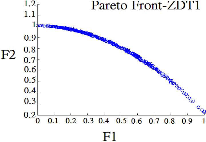
For Definition 4, a Pareto front is represented by each objective function value of every nondominated solution in Definition 3. For instance, like Figure 3.
In MOO problem, we would like to get the Pareto optimal set from feasible set F of all the decision variables vectors satisfied constraints in (2). As noted by Margarita[15], not all the Pareto optimal set is normally desirable or achievable.
Recently, there are more and more evolutionary algorithms (EAs) have been developed in solving MOO problems such as NSGA-II [5], PAES [9], and SPEA2 [19]. These are all population-based algorithms which allow them to probe the different parts of the Pareto front simultaneously.
Particle Swarm Optimization (PSO) was first introduced by Kennedy and Eberhart [10]. It is an algorithm inspired by social behavior of bird flocking. In this algorithm, it will randomly distribute the population of particles in the search space. For every generation, each particle will move toward the Pareto front by the formula of updating velocity, and the best solution for a particle has achieved so far and follows the best solutions achieved among all the population particles.
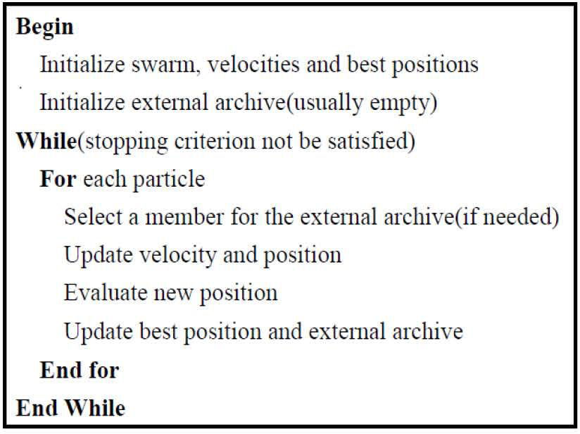
Among those EAs that extend PSO to solve MOO problems is Multi-objective Particle Swarm Optimization (MOPSO) [4], the aggregating function for PSO[16], or Non-dominated Sorting Particle Swarm Optimization (NSPSO) [22]. The Figure 2 shows the pseudocode for MOPSO, this figure shows our optimization algorithm structure.

The MOPSO algorithm we adopt is from [3], which used the concept of crowding distance (CD), and it is called MOPSO-CD algorithm. Note that the formula of updating velocity is stated as:
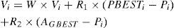
Variables in (4) are:
Vi: velocity
W: inertia
R1, R2 :random number between 0 to 1
Pi: the i- th particle
PBESTi: the i - th particle personal best solution
AGBEST the Pareto best solution in archive
We used the following test problems to verify our implementation is correct.
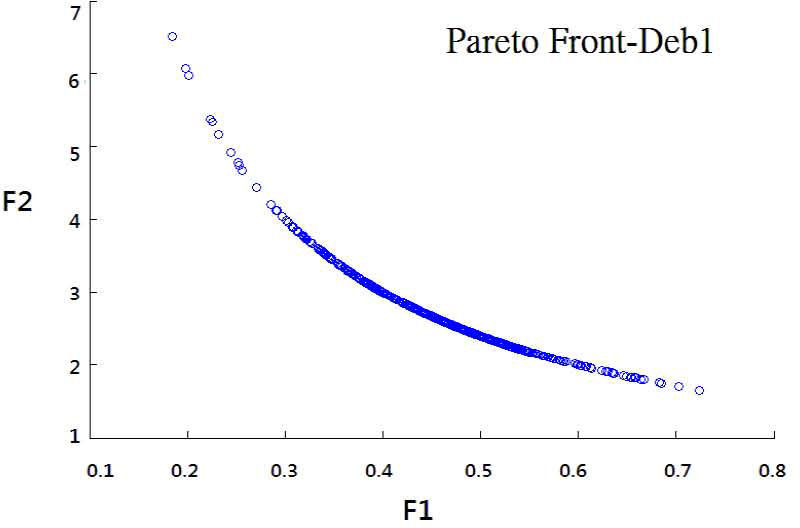
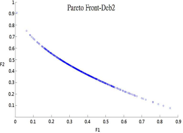
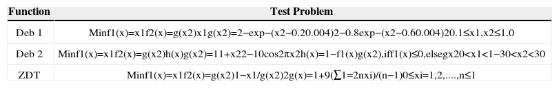
To prove the algorithm feasible, we tried the some famous test problems [6] to test the MOPSO-CD algorithms. Note we also put our input parameters in MOPSO-CD in Table 2. Figure 3 to Figure 5 are the results for problems in Table 1, which can be proved correct in relative research [6].


Test Function for MOO [6]
| Function | Test Problem |
|---|---|
| Deb 1 | Minf1(x)=x1f2(x)=g(x2)x1g(x2)=2−exp−(x2−0.20.004)2−0.8exp−(x2−0.60.004)20.1≤x1,x2≤1.0 |
| Deb 2 | Minf1(x)=x1f2(x)=g(x2)h(x)g(x2)=11+x22−10cos2πx2h(x)=1−f1(x)g(x2),iff1(x)≤0,elsegx20 |
| ZDT | Minf1(x)=x1f2(x)=g(x2)1−x1/g(x2)2g(x)=1+9(∑1=2nxi)/(n−1)0≤xi=1,2,....,n≤1 |
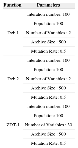
Parameters for Test Function in Table 1.
| Function | Parameters |
|---|---|
| Deb 1 | Interation number: 100 |
| Population: 100 | |
| Number of Variables : 2 | |
| Archive Size : 500 | |
| Mutation Rate: 0.5 | |
| Deb 2 | Interation number: 100 |
| Population: 100 | |
| Number of Variables : 2 | |
| Archive Size : 500 | |
| Mutation Rate: 0.5 | |
| ZDT-1 | Interation number: 100 |
| Population: 100 | |
| Number of Variables : 30 | |
| Archive Size : 500 | |
| Mutation Rate: 0.5 |
In this paper, we use the most prominent large margin for classification tasks SVM. It solved supervised classification problems. A set of data is divided into several classes and this method learns a decision function in order to decide into which class an unseen data should be classified. Because SVM guarantee an optimal solution for given data set, they are now one of mostly popular learning algorithms.
Definition 1[11] Searching hyperplane is defined as:

where w is normal to the hyperplane, is the perpendicular distance of hyperplane to the origin, and ||w|| is the Euclidean norm of w. The vector w and the offset b define the position and orientation of the hyperplane in the input space.
Definition 2The prediction function of new data points is stated as:

This classification problem is to find an optimal hyperplane in a high dimensional feature space by mapping x to ϕ(x).
Traditionally, the problem can be expressed as:

This problem can be solved by evolutionary algorithms [14], however, it has been proved inefficient.
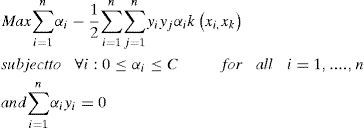
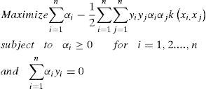
Note that the penalty parameter C in (7) is a user defined weight for both conflicting parts of the optimization criterion. Using positive Lagrange multipliers αi, i = 1,2,...n which is introduced by Wolfe dual [20]. Thus we have the following form:
We then get the optimal vector normal vector:
2.3Multi-objective SVM
We knew that traditional SVM are not able to optimize for non-positive semi definite kernel function. In this paper, we use the formulation from previous research [11] for the reason it can control the over -fitting and omit the penalty factor C, where the two objective functions: maximizing margin and minimizing the number of training errors.
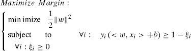
and

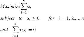
After getting the two objectives, we then can transform both of them into dual forms:
Note that k(xi, xj) is the kernel function, and in our research we used radial basis function (RBF) as kernel function, which expression is k(xi,xj)=exp(−xi−xj22σ2) and used grid search i, j 2cr2 algorithms to determine parameter in RBF.
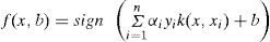
The kernel function k(xi, xj) can be expressed as product of Φ(xi)∙Φ (xj). For non-linear classification problem, the classifier j in (6) can be reformed as the following equation:
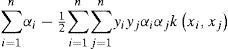
Since both of (12) and (13) share a common term ∑i=1nαi this part of the first objective functions is i=1 not conflicting with the second one in general. We can just omit this term in (12).
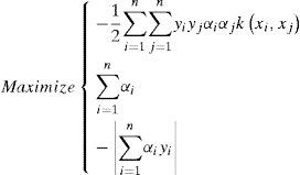
By formulating the problem b = 0, all solution hyperplanes will contain the origin and the constraints ∑i=1nαiyi=0 will just vanish [2]. But if we want the equality constraint to be fulfilled, it can simply be defined a third objective function: −|∑i=1nαiyi| Thus the problem can be reformed as:
By solving (15), we can get the Pareto frontier, yet we still cannot decide which solution on the Paretofrontier is what we need. In previous research, we have two ways to decide the solution: maximum margin model and prediction. Two ways to search the final solution are stated as following:
- •
Maximum margin model: Calculate (16) for particles on Pareto frontier and choose the one with biggest value for result of (16)
- •
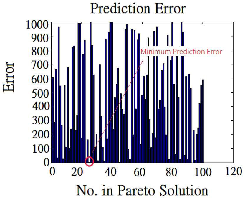
Minimum prediction error: Calculate (17) for particles on Pareto frontier and choose the one with minimum value for result of (17)
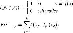
The variable k is for a small hold-out set of the data points of size. These k data points were part of the input training set and are not used by the learner during optimization process. After finish optimization, the learner is applied to all k data points. l(y,f(x)) is just the binary loss, and for p-th particle the errors is Errp. Just plot all errors Errp and compare it with the original Pareto front, and choose the place where the training error and the generalization error are close to each other. This way was proved to control over fitting.
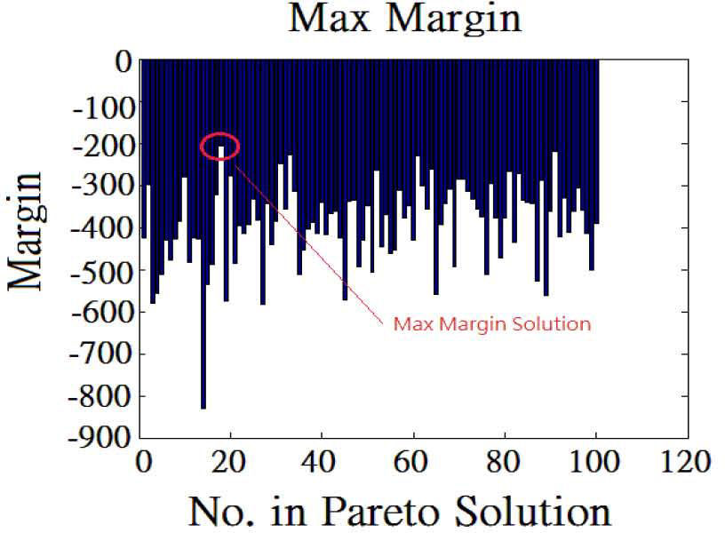
In this study, since there is no research to suggest the appropriate value of k in (17), we try another way to determine the error: use all of training set for MOO process and k is equal to the number of training set samples. In our research, it is proved to be useful in determine the final solution too. This calculation result is shown in Figure. 8 and Figure. 9.
The Figure 8 is Maximum margin for Pareto Solutions in Fig 4. The vertical axis value is the same as Fig. 4 while the horizontal axis is every solution in Fig 4. And the Figure 9 is Prediction Error (in this study) for Pareto Solutions in Fig 4.
The vertical axis value is the same as training error in Fig. 4 while the horizontal axis is every solution in Fig 4. We implement the (15) with MOPSO-CD mentioned in Sec 2.1.
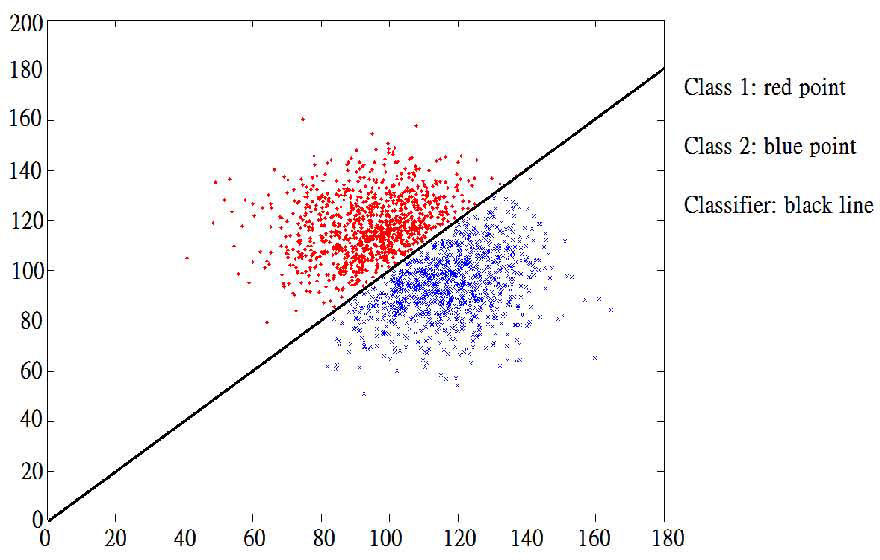
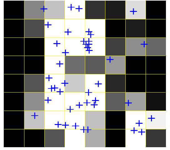
To check if our implementation is feasible, we use 2,000 randomly distributed samples in Figure 6.
.")
The Figure 6 is samples test if the classifier is feasible: the horizontal axis x1 and vertical axis x2 are the a test sample which is composed of (x1, x2).
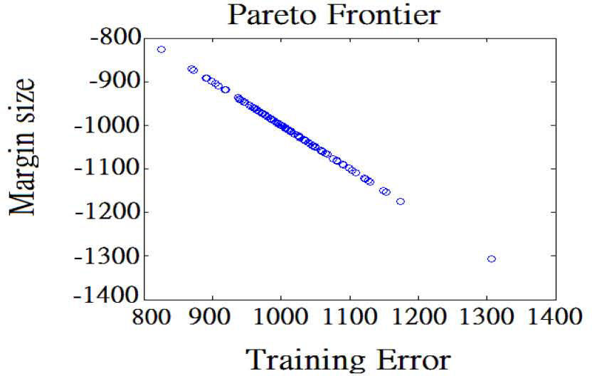
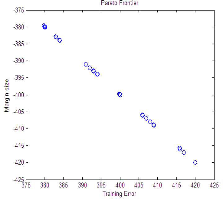
Figure 7 is the Pareto frontier solved for (15), the x-axis is the first objective function, the y-axis is the second objective function and we omit the third objective function in Figure 7 as previous research does. The Pareto frontier for samples results in Fig 3. The vertical axis is margin size calculated by (10) and the horizontal axis is training error which is calculated by (11).

Note that in the original research [11], the author proposed another way to determine solution from the Pareto frontier, which can be shown as following:
- 1.
Separate the training set, take out about 20% set from the training set as a test set.
- 2.
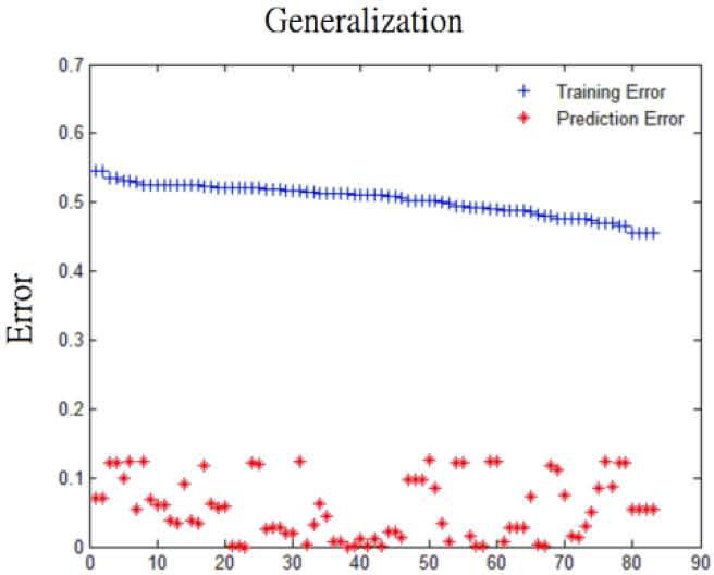
Follow (17) to calculate the prediction error with the result of training error to form another plot, and then user can determine the solution they desired to avoid over-fitting for SVM result.
Follow the above two-steps, we can get Figure 10, this concept is first proposed in research [11], whose author pointed that user could find the position where training error and prediction error are closed by each other to set it as the suitable solution to avoid over – fitting in traditional SVM problem.
Compared with the method we took from Figure 8 to Figure 9, we simply found that we can get the same result for Figure 6, which proved our way feasible and in some cases, more intuitive.

.")
Figure 10 is the way proposed from the original research [27]. It transferred the training error from Fig. 7 and normalized it with total number of Pareto-optimal solutions. As the original authors pointed, this figure can help users to choose solutions without over-fitting for the solution where the training error and prediction error are the closest in the figure. We proposed the way to choose classifier in Fig. 8 and Fig. 9 because in real application, we often just need the smallest prediction error as a pointer and this is more intuitive for user to understand the rule to choose suitable Pareto solution.
 and testing (*) data, and the x-axis denotes a counter over all Pareto-optimal solutions ordered by training errors. Note that all the error is generalized.")
In this example, we generate 100 particles, 100 generations, 100 capacities for extern archive, probability 50% for mutation, and 1.4 for inertia w. By using result from Figure 9, we still can find a good classifier to 100% distinguish two classes. Note that in this example we used the grid search algorithm to determine the of RBF as 0.001.
3Fuzzy encoder on fingerprintTo do the fingerprint classification, we first have to extract features of fingerprints. In our research, we proposed a way to encode the fingerprint image with fuzzy rules. Sec 3.1 shows the way we do the feature extraction, and Sec 3.2 shows fuzzy encoder in our research.
3.1Feature extractionTo obtain higher accuracy, researchers have already investigated various ways such as ridge distributions, directional images or FingerCode [7] and so on. Park [8] used Fourier transform to make an orientation filter. Nagaty [13] extracted a string of symbols using block directional images of fingerprints.
In this study, we took the following steps to extract fingerprint features:
Step 1Normalize the fingerprint image with expression:
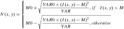
where I(i, j) represents the grayscale value for each pixel, M is the average and VAR is the variance for the image, and N(i, j) represents the grayscale value after normalization. Note that M0 is the expected average while VAR0 is the expected variance. After experiments, we found if we use the number: M0 =127, VAR0 =2000, we can have a best normalization result.
Step 2Image binarization [12]: Since our image is 256 level grayscale image, we should transform it as a image with only 0 and 1.
Step 3Thinning [23]: We did this since we want lines for fingerprint width become only one pixel and retain the original structure.
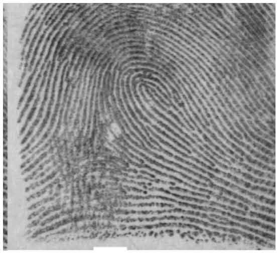
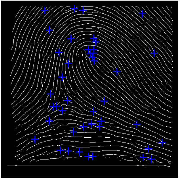
Step 4Minutiae extraction [21]: We followed rules what Simon [21] said and used MATLAB 2010a to get the features of bifurcations and ridges.
Step 5We used two rules [17][18] to ignore the bifurcations.
- •
Ignore the bifurcation if the distance from ridge to it is less than 8.
- •
Ignore one of the bifurcations if distance between two bifurcations is less than 8.
.")

In this section, we will use the result in Sec 3.1 to encode image with fuzzy rules. The goal of developing fuzzy algorithms is to build up a mathematical model to intimate the way people think in logic by computers [24] [25] [26]. In the structure of fuzzy controller, many researchers use the triangular fuzzy member function to define the fuzzy sets.
We used a fuzzy feature image encoder to display the structure of bifurcations in two-dimensional image. This encoder contains three steps:
Step 1Divide a 512 × 512 image into 8 × 8 blocks, which means 8 × 8 fuzzy sets. The radius of each fuzzy set is 64 pixels.
Step 2Define the member function for each bifurcation. The expression is stated as:
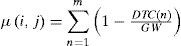
where µ(i, j) is the member function for each (i, j):0 < i < 7, 0 < j < 7
m represents the number of bifurcations in each (i,j), GW means the width for each grid, that is, 64 pixels. DTC(n) is distance of each bifurcation to the center of grid.
Step 3With (19), we can get the fuzzy output for each grid. Theoretically, the value should be between zero to one. Nevertheless, if the density of bifurcations is too big, it might be larger than 1.
Therefore, we define the upper limit to 1. To display the result, we have the following expression:
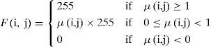
F(i, j) is the grayscale value in each grid.
Follow the above three steps, we make the result Figure 12 into fuzzy image as shown in Figure 13.
4Experimental Results
In this paper, we proposed a new algorithm to transform traditional SVM into multi-objective dual form and use MOPSO-CD algorithm to solve the dual problem. To train the dataset in NIST-4 into our algorithm, we take the fuzzy encoder into a 1x64 array to represent this image sample.
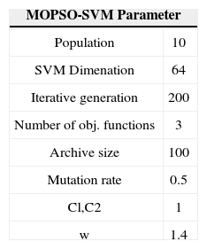
Since there are 2,000 people samples in NIST-4 and each person have 2 fingerprints image. We just pick 1,000 of them as the training set and divide them into two classes, labeled 1 and -1. We used the grid search algorithm to find the is suitable for 1. We set the parameter for MOPSO in the following table
Figure 14 shows the result of optimization problem in this section, we can choose the archive solution by method proposed in section 2.3 to determine the suitable solution. With this solution, we can use it to determine if a new fingerprint is belonged to our database.

Since in our application, there are only two-classes: NIST-4 database or not, we just use the linear multi-objective SVM to testify our training results.
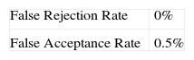
Note that we still can use manual operation to determine the suitable support vector to get result from Table 4, the contribution in this paper is that we proposed a feasible mean to automatically to determine suitable parameters for SVM.
5ConclusionIn this paper, we developed a multi-objective optimized SVM algorithm which is proved effective for binary-class fingerprint classification. This algorithm can reduce the work from manually operation for testing suitable parameters of SVM. Note that even if without our algorithm, people still can spend lots of time building figures in our research. We suggested a more logical and more time-effective way to evaluate the proper SVM parameters compared to other literatures.
However, we did not apply the algorithm to multi-class labeled problem. As a future work, we should put this algorithm forward to applying to multi-class problem.