


Dynamic voltage/frequency scaling (DVFS) is one of the most effective techniques for reducing energy use. In this paper, we focus on the pinwheel task model to develop a variable voltage processor with d discrete voltage/speed levels. Depending on the granularity of execution unit to which voltage scaling is applied, DVFS scheduling can be defined in two categories: (i) inter-task DVFS and (ii) intra-task DVFS. In the periodic pinwheel task model, we modified the definitions of both intra- and inter-task and design their DVFS scheduling to reduce the power consumption of DVFS processors. Many previous approaches have solved DVFS problems by generating a canonical schedule in advance and thus require pseudo polynomial time and space because the length of a canonical schedule depends on the hyperperiod of the task periods and is generally of exponential length. To limit the length of the canonical schedules and predict their task execution, tasks with arbitrary periods are first transformed into harmonic periods and their key features are profiled. The proposed methods have polynomial time and space complexities, and experimental results show that, under identical assumptions, the proposed methods achieve more energy savings than the previous methods.
In the last decade, energy-aware computing has been widely applied not only for portable electronic devices, but also for large systems which incur large costs for energy and cooling. With dynamic voltage/frequency scaling (DVFS) techniques [3, 7, 8, 9, 10, 11, 12, 15, 16, 17, 18, 19], processors can perform at a range of voltages and frequencies. In the CMOS processors, the energy consumption is at least a quadratic function of its supply voltage (and hence the processor frequency) [3, 7, 8, 19, 20, 21], and total energy consumption could be minimized by sharing slack time while satisfying the time constraints of the tasks. For DVFS hard real-time systems, we defined two categories of DVFS scheduling: inter-task DVFS and intra-task DVFS. In the former, speed assignments are determined at task dispatch or completion times. In other words, when an instance (job) of a task is assigned to a CPU, the CPU speed does not change until it is preempted or completed. This definition is somewhat different from the inter-task definition in [3, 13, 16, 20, 23] wherein the speed of each tasks is fixed and cannot be changed between different instances (jobs). Inter-task DVFS scheduling algorithms are often implemented under operating system control, and programs do not need to be modified during their runtime. On the contrary, intra-task DVFS algorithms adjust the CPU speed within the boundaries of a task. Intra-task DVFS techniques are kept under software and compiler control using program checkpoints or voltage scaling points of the target real-time software. It exploits all the slack time from the run variations of different execution paths and the CPU speed is gradually increased to assure the timely completion of real-time tasks. However, checkpoints have to be generated at the compiling time and indicate places in the code where the processor speed and voltage should be recalculated. These checkpoints could increase programming complexity and the overhead of realtime systems. The previous definition of intra-task scheduling [24, 18, 25] is similar to our definition of inter-task DVFS.
Many studies have addressed the problem of task scheduling with minimum energy DVFS. Yao et al. [21] proposed a theoretical DVFS model and an O(n3) algorithm for computing a min-energy DVFS schedule in a continuous variable voltage CPU. Ishihara et al. [14] proposed an optimal voltage allocation technique using a discrete variable voltage processor. However, the optimality of the technique is confined to a single task. Kwon et al. [17] proposed an optimal discrete approach based on the continuous version in [21] and therefore requires O(n3) time. Li et al. [18] proposed an O(dn log n) time algorithm which constructs a minimum energy schedule without first computing the optimal continuous schedule. The abovementioned min-energy DVFS scheduling algorithms have to generate certain schedules in advance as intermediate processing steps. For example, the Bipartition algorithm in [18] has to generate an s-schedule and a reversed s-schedule in advance. Moreover, the Alloc-vt algorithm in [17] has first to generate a min-energy continuous schedule from [21]. Since the lengths of such schedules depend on the LCM of task periods, their algorithms could not be completed in polynomial time. In addition, in the periodic tasks systems, the preprocessing overhead produced by these approaches may become unsustainable when tasks frequently join and leave the system. Many theoretical models for DVFS only consider the power consumption function with convexity [3, 20, 21, 22]. In these models, the processor must be able to run at infinite real-number speed levels to achieve optimality, while an off-the-shelf processor with variable voltages runs only at a finite number of speed levels. For example, Intel’s SpeedStep® technology [25] and AMD’s Cool’n Quiet® [27] are currently used in general-purpose mobile devices and respectively support 3 and 5 speed levels. Therefore, an applicable model for DVFS scheduling should capture the discrete, rather than continuous, nature of the available speed scale.
In network systems, jitter or packet delay variation (PDV) is defined as the variation in the time between successive packet arrivals caused by network congestion, time drift or route changes [19, 28]. PDV is an important quality of service factor to evaluate network performance. One of the most widely-used techniques to improve PDV is pinwheel scheduling [1, 5, 29, 30, 31, 32, 33]. A pinwheel task тi is characterized by two positive integer parameters, an execution requirement and a window-length with the understanding that the shared resource needs to be allocated to task i for at least an out of every b consecutive time units. Pinwheel task systems were developed to meet the performance requirements of satellite-based communications. In more recent applications, broadband 3G (B3G) wireless communication systems provide a packet-switched core network to support broadband wireless multimedia services. The resource management policies in the cell of a B3G system guarantee the quality-of-service (QoS) of real-time (RT) traffic. To guarantee the QoS of RT traffic in a cell, many researchers [1, 2, 5, 4, 29, 32, 34] have proposed using pinwheel scheduling algorithms to reduce the jitter of variable bit rate (VBR) traffic in a cell. In addition, pinwheel scheduling has also been applied in channel assignment policies with buffer and preemptive priority for RT traffic. In other applications, such as the medium access control (MAC) layer of CDMA and TDMA-based wireless networks [19, 35, 36], many pinwheel scheduling schemes have been proposed to solve frame-based packet scheduling problems. These pinwheel methods provide low delay and low jitter for RT traffic and a short-queue length for non-RT traffic.
This paper discusses theoretical power-aware realtime scheduling. We consider a discrete DVFS scheduling problem for periodic task systems given worst-case execution times (WCET). We propose an algorithm that finds a min-energy intra-task DVFS schedule in O(d+k log k) time. An inter-task DVFS method is also proposed, with time and space complexities of O(d+n log n) and O(d+n), respectively. Notations k, n and d respectively denote the number of tasks, jobs and voltage levels. In section 2, we present the model and the notational conventions. Section 3 introduces DCTS and the proposed task profiling algorithms. The DVFS scheduling algorithms are proposed in Section 4. In Section 5, we present the performance analyses of the proposed algorithms and compare the consumed utilization of transformed task sets with those of their original task sets. Section 6 concludes this paper.
2Task modelA pinwheel task Ti is defined by two positive integers, an execution requirement and a window length, with the understanding that the task Ti needs to be allocated to the shared resource for at least a out of every b consecutive time units. In the distance-constrained task systems (DCTS) [13], they stipulated that temporal distance between any two consecutive executions of each job in the pinwheel schedules should always be less than a certain value. DCTS modifies the distance-constraints of longer task periods as a multiplier of a power of two (abbr. to harmonic number) shorter periods, neither of which is longer than its original distance-constraints using the Sr algorithm [13]. The advantage of the period transformation is that the produced schedules have regular start, preemption and finish times, and therefore provide good predictability.
The target model focuses on synchronous, preemptive, and periodic task systems. In the task set т={T1,..., Tk} of k periodic real-time tasks, every task Ti consists of an infinite sequence of jobs ji,1, ji,2,.... A task Ti with a WCET requirement ei and a period pi has a weight wi=ei/pi, where 0<wi<1. A feasible schedule must give each job its WCET between the arrival-time ri and the deadline di. In the task model, we assume that every task period pi and deadline (as well as their distance constraints) has been transformed as harmonic in that they have been sorted according to their periods, p1≤ p2≤...k. Because of the jitterless schedule, the relative beginning bi and finishing time fi of Ti are fixed and can be efficiently obtained in Section 3.
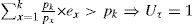
The clock speeds corresponding to d given discrete voltage/speed levels are denoted by s1>s2>...>sd. The highest speed s1 is always fast enough to guarantee a feasible schedule for the given tasks. Moreover, ei and τig respectively denote the duration of the execution at speeds s1 and sg. The time overhead for varying the supply voltage and clock frequency is negligible. In addition, the power loss for the DC-DC converter is also negligible. Let Uτg=∑i=1kwig denote the total weight of tasks in t at speed sg where wig=eig/pi For simplicity, Uτ denotes the total weight of t at the highest speed. The power P, or energy consumed per unit of time, is a convex function of the processor speed. The energy consumed by the processor during the time interval [t1, t2] E(t1,t2)=∫t1t2P(s(t))dt. We refer to this problem as discrete DVFS scheduling (abbreviated to IntraDVFS). The first goal is to find, for any given task set t, a feasible schedule produced by IntraDVFS that minimizes E. In the inter-task version, every job has only one speed during its execution. The second goal is to generate the inter-task (abbreviated to InterDVFS) schedules and to reduce their energy consumption level as close as possible to that of the schedule produced by IntraDVFS.
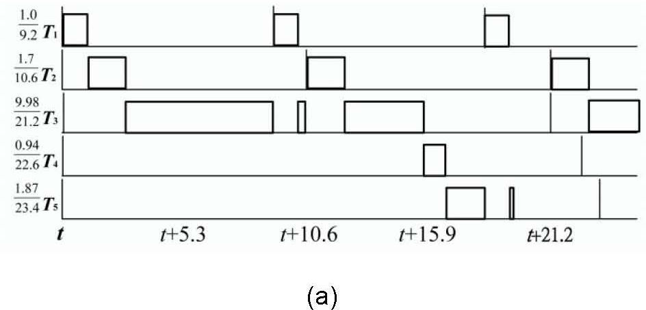
3Distance-constrained task systemsThis section introduces the concept of an h-schedule produced by algorithm Sr mentioned by DCTS [13] and discusses its important properties. Algorithm Sr [31] converts the periods into a set of specialized periods that are not greater than the original periods, while minimizing the increased weight of the total task set. For example, in Fig. 1(a), a system consists of five tasks with periods 9.2, 10.6, 21.2, 22.6 and 23.4, for which the corresponding execution times are 1.0, 1.1, 9.98, 0.94 and 1.87. After applying Sr, the new task periods {5.3, 10.6, 21.2, 21.2, 21.2} are illustrated in Fig. 1(b). Because the lengths of the task periods are multiples of the power of 2, the schedule for each task has no jitter, and their relative starting and ending times are fixed.
3.1Base speed selection Periodic and (b) jitterless schedule.")
 Periodic and (b) jitterless schedule.")
In this section, we prove that any slack time in a jitterless schedule with harmonic task periods can be allocated to all jobs. By using this property, we provide a speed factor for a WCET schedule to minimize energy consumption and the speed adjustment times.
Definition 1An h-schedule, for which τ conforms to the RM policy and the lengths of the task period, is transformed into harmonics using Sr[31].
Without loss of generality, the length of an h-schedule is equal to the longest task period pk. Notably, as long as the utilization of the task set after transformation is less than or equal to 1, the task set can be feasibly scheduled.
Lemma 1Let Uτ≥1; there is no slack time in an h-schedule.
ProofThis lemma is proven by contradiction. Let mi=pk/pi and 1≤i≤k, without loss of generality; we discuss the h-schedule over interval l=[0, pk]. In interval l, the total execution time of tasks in t is denoted as ∑Ti∈tmi×ei.. Assuming that slack time exists in interval l, the following inequality can be satisfied,
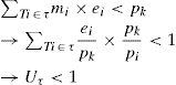
This contradicts our assumption.
Definition 2In the h-schedule for t, we define a deadline as being tight if task Ti finishes just on time at di.
Theorem 2In an h-schedule for t, slack time exists if and only if all jobs in the schedule do not miss their deadlines and the deadline is not tight.
ProofFor the “only if direction, we prove by contradiction.
Case 1(k=1) When an h-schedule contains only one task which has tight deadline, all of its jobs must be finished exactly at their deadlines.
Therefore, no slack time exists in the schedule.
Case 2(k>1) In an h-schedule, all jobs of a task have identical relative finishing times. Without loss of generality, assume Tk has a tight deadline at time t. For all Tx, x, thus it has higher priority than Tk. Because task periods are harmonic, we obtain

mx denotes the power of 2.
Moreover, at the time of t-pk, exactly k tasks are released, and they must have their jobs’ deadlines at the time of t. Therefore, for all Tx, the execution time of their jobs that complete over the interval [t-pk, t] can be written as follows:
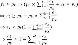
Since we have assumed fk≥ pk and pk×∑x=1k−1expx+ek,
Without loss of generality, Tk has the lowest priority in t and we derive Uτ≥ 1. According to Lemma 1, this contradicts our assumption.
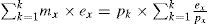
The proof of the “if” direction is easily found. Suppose the h-schedule for τ contains no slack time. Without loss of generality we only discuss the jobs performed in interval l. The total execution time of these jobs can be written as: ∑x=1kmx×ex.. Since interval l contains no slack, we have:
When a Uτ>1, h-schedule is not feasible, at least one job is missing its deadline. When Uτ =1, the latest job in interval l must have a tight deadline.
This completes the proof.
Based on Theorem 2, as long as an h-schedule that is executing at a constant speed is missing a deadline or has a tight deadline, there is no wasted slack time in the schedule. We define the suitable processor speed for h-schedule as follws:
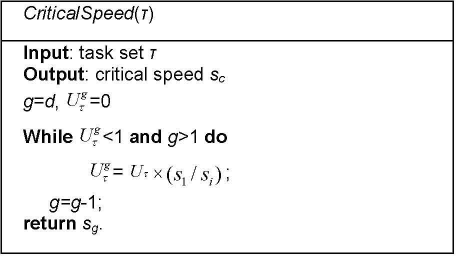
Definition 3In an h-schedule for τ, we define the critical speed sc as the highest speed such that all tasks execute at speed sc and Uτc≥1.
The function of speed sc produced by CriticalSpeed(t) in Fig. 2 generates the base speed for the tasks to produce a suitable h-schedule and to reduce the number of speed adjustments.
3.2Task execution profiling
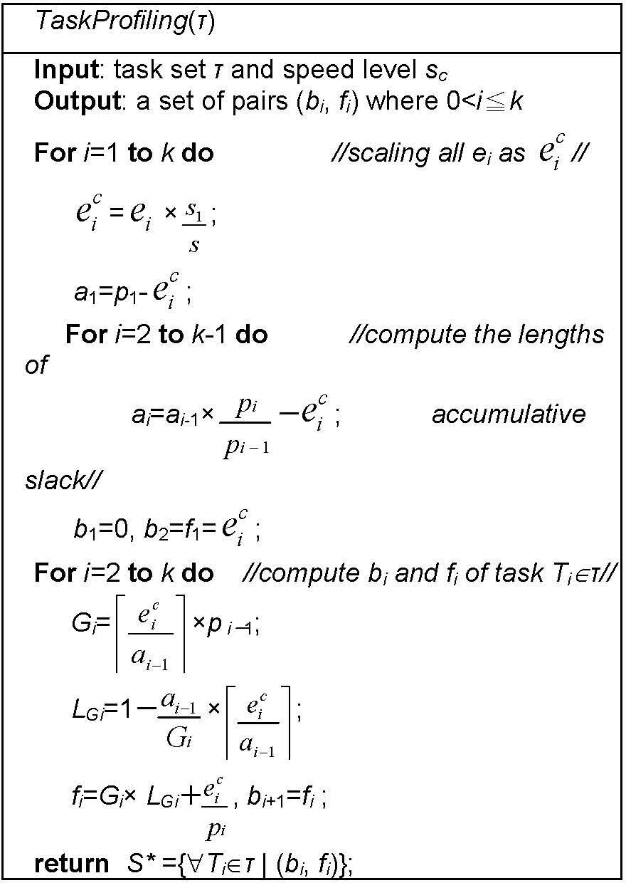
After computing sc, the beginning and finishing times of each task under speed sc can be derived without constructing an actual h-schedule. In Fig. 3, Algorithm TaskProfiling obtains bi and fi of all the tasks that are in O(k) time.
4Scheduling algorithms
For an h-schedule under speed sc, we define the following:
εc: the length of execution time that exceeds pk and is derived from Uτc−1×pk.
δ: the shortest execution time under execution speed sc−1 that prevents an h-schedule under speed sc from missing deadlines and denotes ϵc×sc−1sc−1−sc
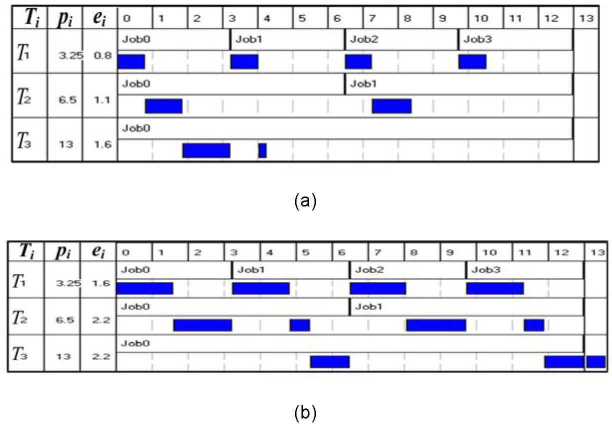
For example, in Fig. 4(a), we can derive ϵc=Uτ3−1×p3≅1 and δ=ϵ3×s2s2−s3≅2.67. That is, the h-schedule in Fig. 4(b) has to increase the speed of an interval of at least 2.67 in length from s3 to s2 to ensure deadlines are met.
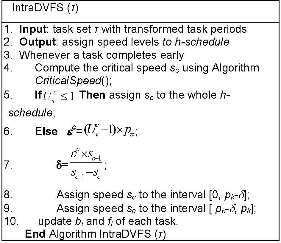
4.1Proposed algorithm for the intra-task schedule

Figure 5 presents an DVFS algorithm for the intra-task schedule, which minimizes the number of speed/voltage transitions and energy consumption.
Theorem3An h-schedule for task set τ consumes the minimum energy using the IntraDVFS (t) algorithm.
ProofAn h-schedule with minimum energy consumption has no idle period. In the algorithm IntraDVFS(t), energy consumption under speed sc and sc-1 is determined by the total processor run time. According to lines 8 and 9 in IntraDVFS (t), an h-schedule with WCET clearly contains no idle period. Moreover, because of the convex property of the function related to power speed, the wide-gapped speed adjustments will make it difficult to obtain significant energy savings [43]. Consequently, the range of speed adjustments of the IntraDVFS (t) is at most one speed level, when an h-schedule under speed sc misses a deadline. Therefore, the speed adjustment for h-schedule minimizes energy consumption, and this completes the proof.
The algorithm in Fig. 5 has a time complexity of O(d+k log k) time, where k denotes the number of tasks in τ. In the algorithm, its input periods have to be transformed in advance by Sr [19], which runs in O(k log k) time, and line 3 in algorithm CriticalSpeed() needs O(d) time to find a critical speed. Notably, the time complexity of the algorithm in [30] is O(dn log n) where n denotes the number of jobs. In a task system, the number of jobs is far greater than the number of tasks. Therefore, our scheme outperforms their algorithms, even if we ignore the overhead incurred by producing the whole schedule in the method presented in [30].
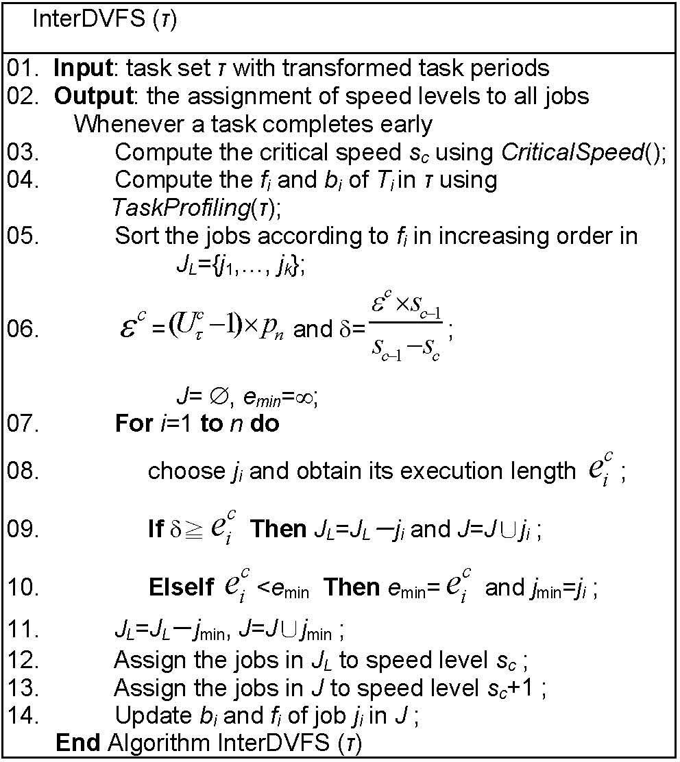
4.2Proposed algorithm for the inter-task schedule
In an h-schedule produced by a InterDVFS (t), each job has a unique execution speed whenever it performs. However, the decision for speed adjustment is similar to that of the knapsack problem with an unbroken object and identical value. More precisely, given that δ is derived from the h-schedule, we have to decide which jobs can be placed into the interval in such a way that the sum of their execution time is greater than δ and their differences are minimal. Unfortunately, the optimization algorithm for this decision problem runs in pseudo-polynomial time [14]. In other words, the time complexity depends on the length of an output schedule.
The objective of our algorithm is to minimize the fluctuation of execution speeds. Thus, the proposed method has to know the task profiles produced by Algorithm TaskProfiling( ) in Fig. 3. Jobs are arranged in order of increased speed by sorting all jobs by their finishing times and therefore interDVFS takes O(n log n) time. In Fig. 6, from lines 7 to 10, we they search for suitable jobs according to this order and book the nearest job with the minimum execution time, thus the time complexity is at most O(n). For the time complexity of the rest of algorithm InterDVFS( ), the remaining period transformation takes O(k log k) time, finding the critical speed takes O(d), and computing the values of fi and bi of each task takes O(k). In general, the value of n is much larger than that of k in a periodic task model, and the running time of algorithm InterDVFS( ) is O(d+nlogn).
Example
In Fig. 4(c), the first job of T1 is included in job set J due to the for-loop in algorithm InterDVFS( ). In line 12, the second job of T1 is finally assigned to jmin and included in J.
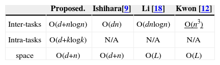
5Performance analysisWe discuss the performance of the techniques proposed in [14, 17, 18, 21]. Because the methods belong to intraDVFS scheduling and are optimal power consumption solutions, we can only compare their time complexities.
The levels of complexity for the given methods are shown in Table 1. The second and third rows present the time complexities of InterDVFS and IntraDVFS techniques. Notations n, k and d respectively denote the numbers for job, task and speed levels. Notably, L denotes the length of an input schedule. In a periodic task system, the number of jobs is far greater than that of tasks and our intraDVFS algorithm outperforms the others.
Notably, the method proposed by Ishihlara et al. is formulated as a linear programming problem and has at least O(dn) time complexity [12]. However, the optimality of the technique is confined to a single task. Therefore, the optimality does not hold for the practical case in which every task has different execution speeds. In addition, the techniques proposed in [16, 18] have to generate a “canonical” schedule before voltage/speed adjustments. The memory space required by the above-mentioned methods is dominated by the length of such schedule and cannot be generated in polynomial time.
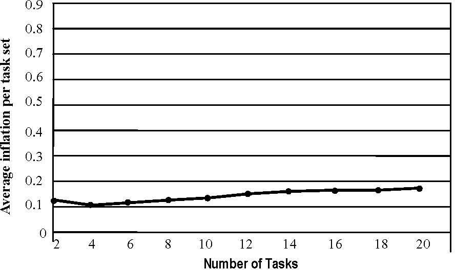
The simulations results in Fig. 7 presentes the inflation of UT caused by Sr and (2) the energy-efficiency of interDVFS scheme. Because of period transformation, UT is greater than its original utilization and the difference between them is called inflation. In Fig. 7, Sr is performed in the 20,000 randomly generated task sets with varying sizes. For example, when every т contains 6 tasks, the average inflation per task set is 0.14. The figure indicates that inflation will rise at a rate proportionate to the size of task set.

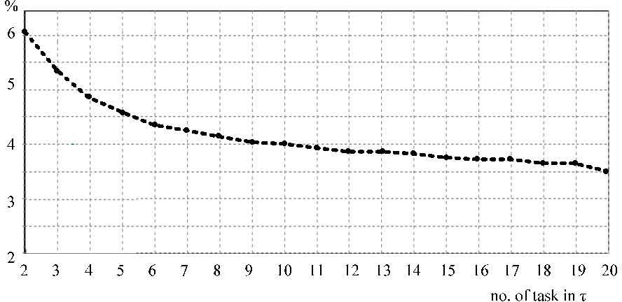
Since the intraDVFS scheme produces a min-energy schedule, it can serve as a yardstick by which to assess the energy efficiency of interDVFS. Figure 8 presents the percentage of the normalized deviation produced by interDVFS as compared to that of the optimal solution versus task set size. Because previous works [9, 12, 14, 15] optimized energy consumption, no comparison need be made with the proposed interDVFS. The figure shows the energy consumption of interDVFS does not deviate more than six percent from that of the optimal solution. It also indicates that energy consumption is rather sensitive to variation of task set size. The deviation is less than 4% when task set size is greater than 10. The main reason is that, when the number of tasks increases, the number of candidate tasks to share the slack time is also increased.

In additioin, we evaluate the effectiveness of InterDVFS on randomly generated task sets and compare its energy consumption with DRA, AGR [1] and lpSHE [13]. Both DRA and AGR are modified to account for time transition overhead. Each task is characterized by its worst-case execution wci, its period pi, and its deadline di, where di=pi. We vary three parameters in our simulations: (1) number of tasks totaltasks in т from 2 to 20 in two task increments, (2) the probability of an early completion (prob. of EC) for each job, and (3) the bc/wc ratio of BCET to WCET, from 0.1 to 0.9. For any given pair of totaltasks, U and bc/wc in T, we randomly generate 1000 task sets, and the experiment result is the average value over these 1000 task sets. In a task set, each task period pi is assigned randomly in the real number range [1, 100]ms with a uniform probability distribution function. The execution time wci of each task is assigned in the real number rang [1, min{pi−1, 450}]. After giving the values of tasks’ periods and executions, we assign the utilization U of a task set and rescale the pi of each task such that the summation of the task weights (i.e. wci/pi) is equal to a given U. The early completion time of each job in simulations (1) and (2) was randomly drawn from a Gaussian distribution in the range of [BCET, WCET], where BC/WC=0.1. In simulation (3), each experiment was performed by varying BCET from 10% to 90% of WCET. The experiment calculates the energy consumption of each task set in an interval of time l=2000. After generating the task set, a duplicate of the task sets are transformed to have powers of 2 periods. Therefore, the duplicate has higher actual utilization than initially intended. In the period transformation tasks, since the simulation tasks still complete early proportionately according to the experiment settings, the slack originated from additional utilization still be utilized by slack-time analysis algorithms.
The processor model we assumed is base on the ARM8 microprocessor core. For all experiments we assume there are 10 frequency levels available in the range of 10MHz to 100MHz, with corresponding voltage levels of 1 to 3.3 Volts. The assumption of voltage scaling overhead is the same as that in [24], and an idle processor consumes at most 500μW at the processor sleep mode. The energy consumptions of all the experiment results are normalized against the same processor running at maximum speed without DVFS technique (non-DVFS). Table 2 is a summary of our simulated ARM8 processor core [37].
The overheads considered in the simulations are as follows.
(1) Algorithm execution time and energy
The energy overhead is obtained under the assumption of 80% of the maximum power [24].
(2) Voltage transition time and energy
The assumption of voltage scaling overhead is the same as that in [24] and the transition time is at most 70us between maximum transitions [38]. The energy consumed during each transition is:

where λ denotes the efficiency of DC-DC converter.
For the voltage scaling from Vdd1 to Vdd2, the transition time is:
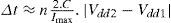
where C and lmax denote the charge to the capacitor and the maximum output current of the converter.
(3) Context-switch time and energy
The context-switch is assumed to be 50μs at the highest speed Smax as presented by David in [40].
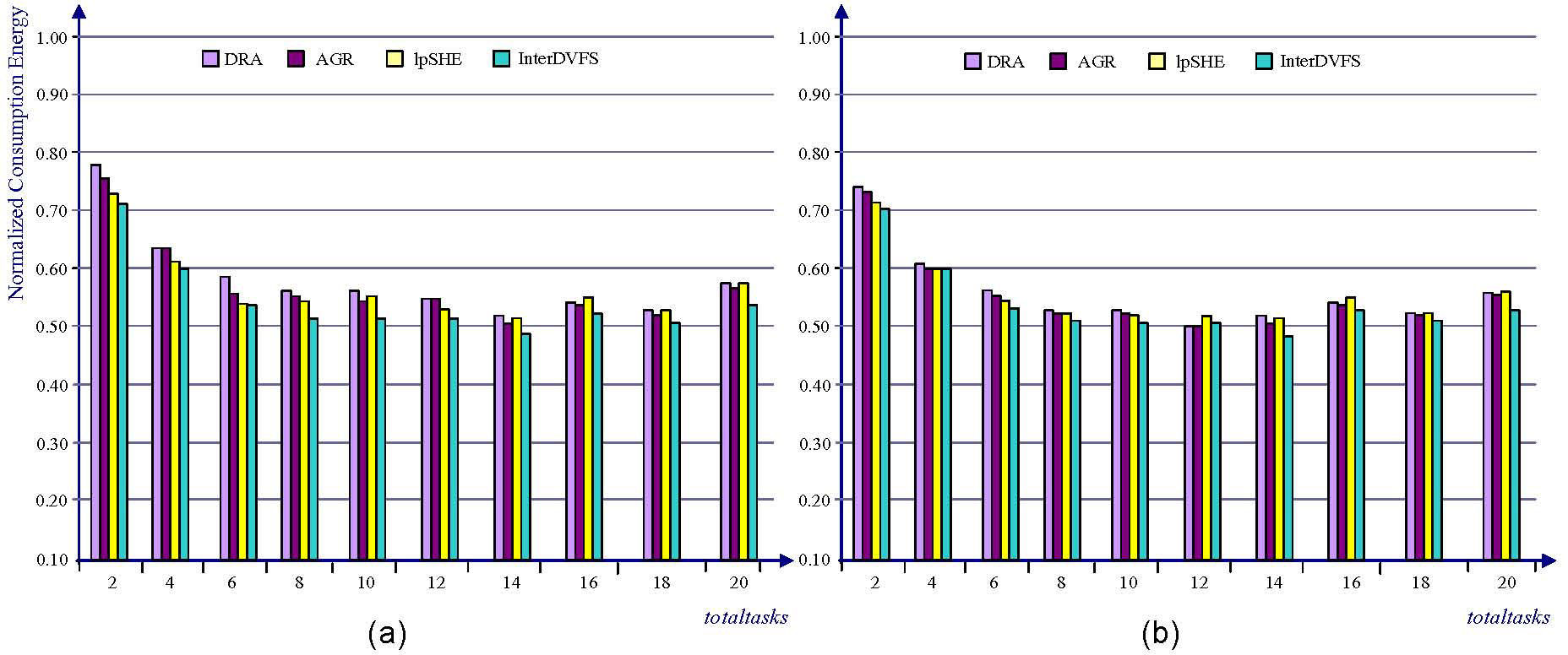
Figures 9 (b), 10 (b) and 11 (b) have been done under the assumption that the lengths of task periods in the non-DVFS, DAR, AGR and lpSHE are transformed to the power of 2, while those in Figures 9 (a), 10(a) and 11 (a) are not transformed. As shown in Figure 9 (a), InterDVFS reduces the energy consumption up to 5% over DRA. The utilization of a given task set is 60%. As the number of tasks from 8 to 20, the energy consumption of InterDVFS is increased steadily. The reason for this fact is that InterDVFS focuses on distributing the slack on as many tasks as possible. When the number of tasks increases, the available slack can be shared by many tasks due to the jitterless schedule. Therefore InterDVFS decreases the number of speed/voltage scaling and benefits the energy saving. In Figure 9 (b), DRA, AGR and lpSHE have closer energy consumption with each other than those in Figure 9 (a). InterDVFS still outperforms other methods especially in the large totaltask.
 tasks without period transformation and (b) tasks with period transformation (U=60%, bc/wc=0.5).")
 tasks without period transformation and (b) tasks with period transformation (20 tasks, U=60%, bc/wc=0.5).")
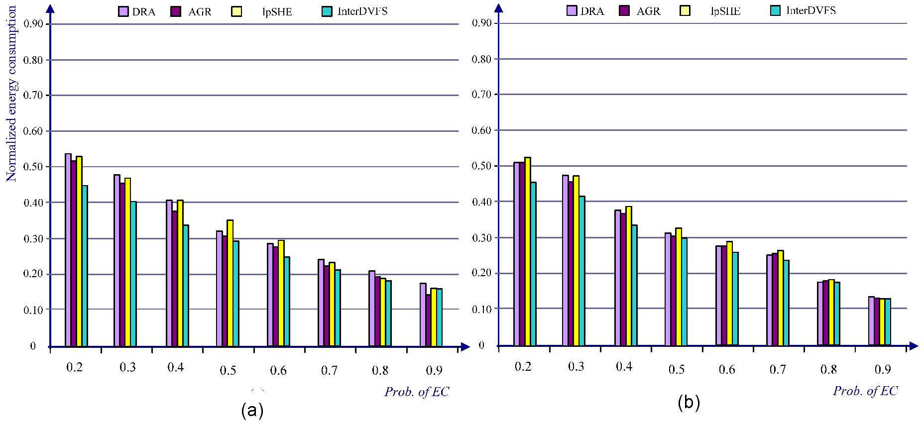
 tasks without period transformation and (b) tasks with period transformation (2~20 tasks, U=60%, prob. of EC is 0.5).")
In Figure 10(a), when prob. of EC is smaller than 0.8, InterDVFS performs 2%~12% more energy saving compared to AGR and DRA. When prob. of EC is 0.9, the results are not good as we had hoped, they are 7% worse than those of AGR. In the experiment, the totaltasks of each task set is randomly determined from 2 to 20. As the probability of early completion decreases, the differences between InterDVFS and DRA or AGR increase substantially. On the contrary, when the largely jobs complete early, the amount of current available slack would be changed frequently and the voltage levels of other related jobs have to be changed. The harmful effects of frequently voltage change compromise the advantage of InterDVFS that benefits the evenly distribution of slack. In Figure 10(b), InterDVFS still outperforms up to 8% energy saving compared to other methods.
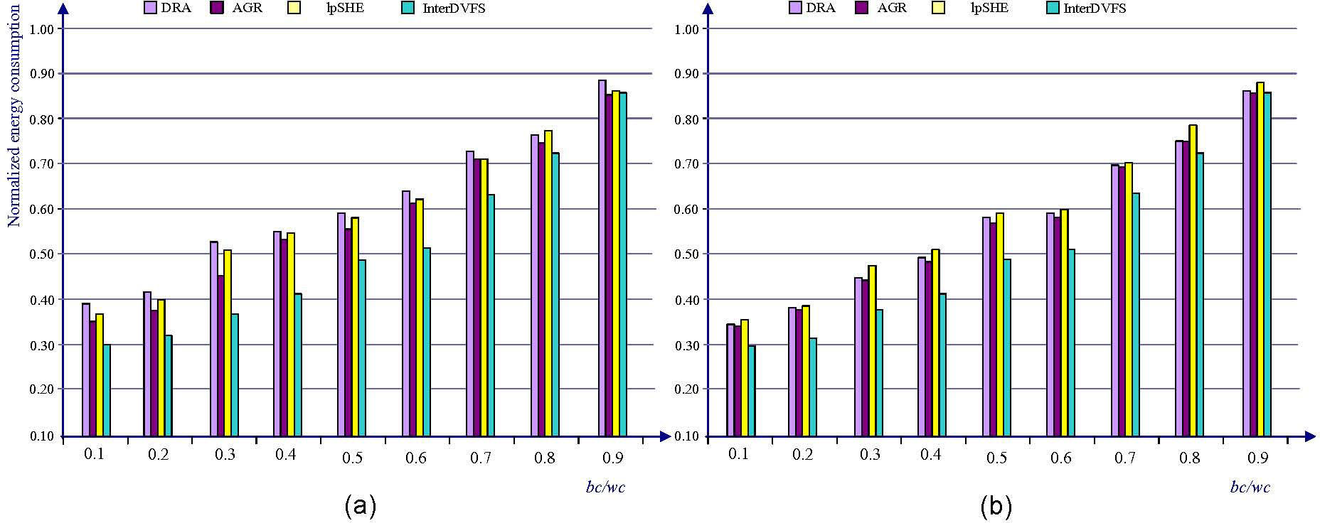
The effect of bc/wc shown in Figure 11(a) and 11(b) confirms our prediction that the energy consumption (U=0.8, prob. of EC is 0.5) would be highly dependent the variability of the actual workload. When bc/wc=0.9, the energy consumptions are quite close for all four techniques, as expected. However, once the actual workload decreases, the algorithms are able to reclaim slack time and to save more energy. Algorithm InterDVFS gives the best energy saving, followed by AGR DRA and lpSHE. Decreasing the ratio helps further improve the relative performance of InterDVFS due to the equally assigned voltage/speed level to the future jobs.
In a jitterless schedule, more jobs have the same release times and deadlines as those in the schedule with original periods. Therefore, the appearances of next task arrival (NTA) become regular and the distances between NTAs are longer than that in the schedule without period transformation. At each scheduling point, when the distances between each pair of NTAs are longer, DRA, AGR and lpSHE obtain more energy savings. This is because they can derive longer slack between the NTAs. In addition, when more tasks release at the same time, they can predict the length of slack more precisely and easier. As the example shown in Figure 1(b), a schedule without jitters makes more jobs share available slack than those generated by original periods. Although InterDVFS has the penalty for utilization inflations, it still outperforms other techniques.
Since non-DVFS does not as sensitive as DRA, AGR and lpSHE to period transformation, its energy savings is modest while other methods have relatively less energy consumption. It is likely to that these methods gain more savings by predicting the length of slack in the future interval. Moreover, in the Figures 9(b), 10(b) and 11(b), the energy consumptions of DRA, AGR and lpSHE are closer with each other than those without period transformation in Figures 9(a), 10(a) and 11(a). The experiments show that jitter-controlled schedule can decrease the energy consumptions of up-to-date DVFS algorithms. Therefore, it is a promising technique in many real-time applications.
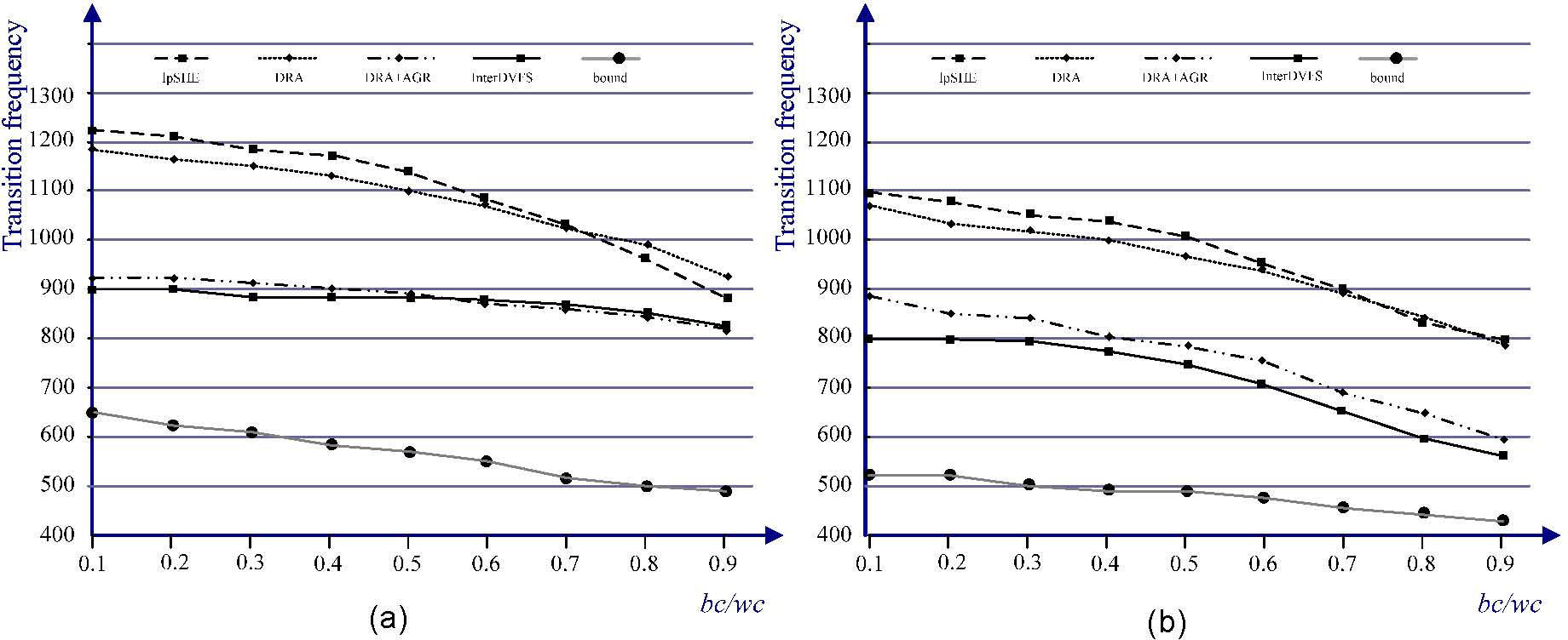
Figure 12 shows how the number of speed transition changes with the DVFS algorithms. The number of transitions is measured with varying the rates of bc/wc. The length of generated schedules and task periods is up to 2000ms and 100ms, respectively. Figure 12 also considers the results for a clairvoyant algorithm, named bound, which checks all possible scheduling points in the whole schedule as well as looks for the best speeds, start and completion times. In fact, bound is extremely time-consuming for finding a combination with the minimum transition times. The results illustrate that lpSHE, DRA and AGR have higher frequencies of transitions than that of InterDVFS
6Conclusion Average Transitions for the task sets versus bc/wc at U=0.5 and d=10 and (b) Average Transitions for the task sets versus bc/wc at U=0.5 and d=4.")
In this paper, we consider the pinwheel task model on a variable voltage processor with d discrete voltage/speed levels. On the assumption of harmonic task periods, we propose an intra-task scheduling algorithm which constructs a minimum energy schedule for k periodic tasks in O(d+k log k) time. We also propose an inter-task scheduling algorithm which decreases the number of speed or voltage switching events in O(d+n log n) where n denotes the number of jobs. Our schemes outperform the scheme in [18] even though the number of tasks is equivalent to that of given number of jobs. Moreover, since the schedule is obtained without generating an actual schedule in advance, our schemes are true polynomial time algorithms. We also propose some fundamental properties associated with jitterless schedules which may provide new insights for jitterless tasks scheduling.
Aknowledgments
The author would like to thank the National Science Council of the Republic of China, Taiwan, for financially supporting this research under Contract No. NSC 102-2221-E-025-003.