Feature-based fast coding unit partition algorithm for high efficiency video coding

Abstract

High Efficiency Video Coding (HEVC), which is the newest video coding standard, has been developed for the efficient compression of ultra high definition videos. One of the important features in HEVC is the adoption of a quad-tree based video coding structure, in which each incoming frame is represented as a set of non-overlapped coding tree blocks (CTB) by variable-block sized prediction and coding process. To do this, each CTB needs to be recursively partitioned into coding unit (CU), predict unit (PU) and transform unit (TU) during the coding process, leading to a huge computational load in the coding of each video frame. This paper proposes to extract visual features in a CTB and uses them to simplify the coding procedure by reducing the depth of quad-tree partition for each CTB in HEVC intra coding mode. A measure for the edge strength in a CTB, which is defined with simple Sobel edge detection, is used to constrain the possible maximum depth of quad-tree partition of the CTB. With the constrained partition depth, the proposed method can reduce a lot of encoding time. Experimental results by HM10.1 show that the average time-savings is about 13.4% under the increase of encoded BD-Rate by only 0.02%, which is a less performance degradation in comparison to other similar methods.

1

Introduction

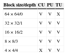
With rapidly increased demand for higher visual quality in consumer devices, the video coding standard H.264/AVC has been becoming insufficient in terms of rate-distortion coding performance. The new HEVC (or called H.265) standard was established by ITU-T VCEG and ISO/IEC international organizations to meet the newest visual coding requirements for ultra high definition videos (Sullivan, Ohm, Han, & Wiegand, 2012). HEVC employs a quad-tree based coding block structure to increase the rate-distortion performance. The types of quad-tree block defined in HEVC include CU, PU and TU blocks. The CU in HEVC is the basic coding block, similar to the macroblock in H.264/AVC, except that CU could be split further into PU and TU blocks in HEVC. The role of PU is to help get a good prediction of image blocks based on a predefined set of 35 prediction modes. And TU is a partition of prediction residue for a CU in order for obtaining better DCT/DST transform performance. Table 1 shows that the possible block sizes of CU, PU, TU and the corresponding distinct quad-tree depth, respectively. The symbol “V” represents the size supports for the block type and “X” means not supported for the block type.

Table 1.

Block sizes for different block types.

Block size/depth	CU	PU	TU
64 × 64/0	V	V	X
32 × 32/1	V	V	V
16 × 16/2	V	V	V
8 × 8/3	V	V	V
4 × 4/4	X	V	V

Figure 1 shows an example of quad-tree partition for a block of 64 × 64 pixels, in which it should execute 341 times process of PU, TU and encoding for the incoming block. A lot of encoding time is required for this coding process, and then it limits the possibility of HEVC in real-time applications. There are some fast algorithms proposed to speedup the HEVC encoder. Lee, Kim, Kim, & Park (2012) introduces the co-located CU in previous frame to predict the quad-tree depth of current encoded CU block. Cheng, Teng, Shi, & Li (2012) and Shen, Liu, Zhang, Zhao, & Zhang (2013) apply neighbouring CUs and parent CU information of quad-tree partition to estimate the possible split of current block and prediction mode of intra coding, which can provide up to 40% and 20% time-savings, respectively. Shen et al. (2013b) and Zhang, Wang, & Li (2013) present the neighbour reference method to decide the CU depth level in the inter coding mode. These methods can easily and quickly achieve the time-savings and the compression ratio. However, in some cases, the estimation is not always accurate. For example, in frames with fast moving objects or blocks located at frame boundary (Fig. 2, green rectangles) do not have reliable adjacent reference blocks for estimation. This means that there is no significant time-savings on these blocks. In order to solve the above-mentioned problem, the non-reference adjacent block information method was proposed. Some methods adopted RDCost (rate-distortion cost) to early terminate the split of CU (Kim, Jun, Jung, Choi, & Kim, 2013; Zhang & Ma, 2013). They used RDCost and threshold values to derive the most probable split of block. The average time-savings is up to 20% and 60%, respectively. Zhao, Shen, Cao, & Zhang (2012) employs QP (quantization parameter) value to decide the possible block depth level. Choi and Jang (2012) utilized the nonzero DCT coefficients in TU to terminate the determination of TU partition. Other methods were proposed to reduce PU partition options and prediction modes. For example, Yan, Hong, He, & Wang (2012) proposed to utilize RMD to reduced RDO calculation. Da Silva, Agostini, & da Silva Cruz (2012) and Jiang, Ma, & Chen (2012) also present the filter-based algorithm to find the best intra prediction mode. These methods are accompanied with different thresholds to terminate the calculation. But they do not require the neighboring block information.

Fig. 1.

Quad-tree coding partition example.

Fig. 2.

Boundary partition blocks.

As for the determination of threshold values, there are two categories of method: adaptive and non-adaptive. The adaptive threshold method is able to vary threshold values during the coding process in accordance with the variation of video content. It has a higher practicability to account for the variation in videos. The non-adaptive threshold method uses fixed threshold values for a single video coding process. The thresholds are usually determined from extensive experiments and analysis. This approach would has a best compression and time-savings in particular sequence. This paper focuses on the non-adaptive threshold method. The thresolds are varied with QP values setting before encoding each video.

This paper proposes a fast feature-based algorithm for CTB depth level estimation. The concept of the proposed method is based on our previous work (Lin & Lai, 2014) that uses image features to early terminate the partition process of CUs for speeding up the HEVC encoder. For image processing, image features can really provide effective tools for estimating the visual content of pixels in an image patch (Yasmin, Sharif, Irum, & Mohsin, 2013;Yasmin, Mohsin, & Sharif, 2014). In this paper, an in-depth elaboration of how feature-based CU partition employs image features to speedup CU partition and an extensive experiment are provided to evaluate the fast feature-based CU partition method. In the subsequent parts, Section 2 introduces the HEVC intra coding process. Then, Section 3 presents the proposed fast algorithm method. Section 4 shows the experimental results and makes comparison to another method. Finally, Section 5 concludes the paper with remarks and future works.

2

HEVC intra coding process

Figure 3 shows a block diagram of the HEVC encoder architecture. Firstly, it divides the incoming frame into a set of CTB blocks and encodes each CTB at a time in the subsequent functional blocks. The main function of intra coding lies in the block intra-prediction to remove the redundancy among spatial neighboring pixels in a single video frame. The intra prediction of HEVC employs different angular prediction modes to make smaller prediction residual signal for the block. On the other hand, the inter coding implements the motion estimation and motion compensation to generate a better prediction of blocks with referring to temporally neighboring pixels across neighboring frames. This approach is similar to the inter coding part of H.264/AVC. Finally, the prediction result and the associated prediction parameters are transfered to entropy coding functional block to complete the encoding of the frame.

Fig. 3.

HEVC encoder diagram.

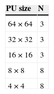
In this section, the intra coding process in HEVC is mainly described. As shown in Figure 4, the incoming frame is firstly split into a series of 64 × 64-blocks, each of which is called the largest CU (LCU) and would be processed individually in the encoder. In intra mode prediction, HEVC provides 35 angular prediction modes (Fig. 5, bottom-left) for predicting current CU by using its neighboring pixels. The HEVC standard defines the rough mode decision (RMD) process (Piao, Min, & Chen, 2010) to reduce the 35 prediction modes into N candidate modes before getting the best prediction. The possible values of N are defined by Table 2. For the larger CU, such as larger than 16 × 16 size, N is set to a smaller value of 3; otherwise, N is 8. The rate-distortion optimization (RDO) process performs to select a best mode from the N candidate modes.

Fig. 4.

64 × 64 split on the frame.

Fig. 5.

Quad-tree coding structure and 35 prediction mode in intra coding.

Table 2.

N candidate modes.

PU size	N
64 × 64	3
32 × 32	3
16 × 16	3
8 × 8	8
4 × 4	8

To obtain a possibly better RD performance, the LCU is tried to be partitioned into four smaller blocks (Fig. 5, upper-left) for examining their individual RDCosts. If the sum of the RDCosts by the four child blocks is found to be less, this CU is decided to be partitioned and the associated SplitFlag is set to 1; otherwise the current CU is keep intact and the SplitFlag is assigned a value of 0. This partition and decision process is repeated until the CU size reaches 8 × 8. At this stage, the 8 × 8-PU and its four 4 × 4-PUs are evaluated to determine the RDCost of 8 × 8-CU and the SplitFlag value. For clarity, the left-part of Figure 5 demonstrates a conceptual example of recursive quad-tree partition from depth 0 to depth 3 for a LCU sized of 64 × 64 pixels, which is called CTB for its encoded results.

Figure 6 shows the encoding process for each CTB in the HEVC intra coding mode. The variable i indicates the position of the four child blocks in a partitioned CU. The meaning of its each value, 0, 1, 2, and 3, is defined in Figure 6B. In the partition process, the variable d is used to denote the depth of current quad-tree partition. With the depth-first partition manner, p(d) is used to store the position number i of all the parent blocks in the partition path starting from the root node that are being encoded currently. C(d, i) records the RDCost value for the i-th CU at depth level d in the partition path. SplitFlag(d, i) records the split status. When this flag is one, it means the CU is split into four equal size blocks in depth d of block i; otherwise, it is combined as a single larger block. The step-wise explanations of Figure 6 is stated as follows:

• •

  Step 1. Initial parameters: i=0; d=0.

• •

  Step 2. Perform the intra coding of i-th sibling CU. This step encodes the CU with the best RDCost stored in C(d,i).

• •

  Step 3. If the depth d of current CU is less than 4, go to Step 5.

• •

  Step 4. If there exists other sibling (i) CUs of current CU block, let i=i+1 and go to Step 2; otherwise, go to Step 6.

• •

  Step 5. Let p(d)=i, i=0 and d=d+1, then split current CU into four child CUs and go to Step 2 to perform intra mode prediction for them.

• •

  Step 6. Let d=d-1, i=p(d) and move up to the parent CU (i-th) to see if the parent CU should be split or not. If d is 0, then end the split process; otherwise go to Step 4.

Fig. 6.

Procedure of CTB encoding process.

3

Feature-based CU partition algorithm

The proposed CU partition algorithm exploits the relationship of image edge feature with the CU size to reduce the number of quad-tree partitions for each incoming LCU or CTB. In the following subsections, the proposed algorithm and the image feature that is used are described.

3.1

Edge features versus quad-tree partition

In natural videos, it is easily found that the smaller blocks in a quad-tree partitioned frame are usually located in the complex edge region of video scene. For example, as demonstrated in Figure 7 for BQSquare_416 × 240 sequence coded in QP 32, the smooth image patches are partitioned with larger block (Fig. 7B), while Figure 7C shows a complex image patch partitioned with smaller blocks (higher depth partition). In accordance with this observation, it is speculated that image edge feature in a CU is highly related to the block size of partitioning it by the quad-tree structure. And it motivates the development of fast CU partition algorithm in this paper.

Fig. 7.

A: Partition example of CTB in BQSquare sequence. B: weak edge. C: strong edge.

3.2

The definition of image edge feature

The edge feature in each LCU is used in the proposed algorithm. To measure the edge feature, Sobel edge detectors (e.g., Fig. 8) is employed to calculate the edge strength in LCU.

Fig. 8.

Sobel edge detectors.

For pixel at (i, j) in any 16 × 16-subblock of LCU, its horizontal-direction and vertical-direction egde components are calculated as follows:

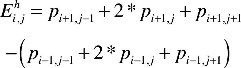
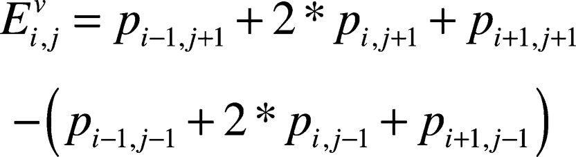
where 0 < i,j < 16. The and represent the pixel edge components in vertical and horizontal directions respectively, is the pixel value at position (i,j) in the LCU. The amplitude or strength of edge pixel is defined in Eq. (3) and represented by A_i,j.

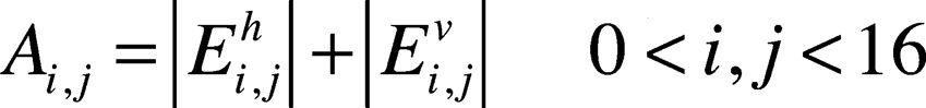
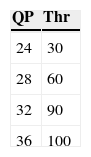
If A_i,j is found to be greater than a pre-specified threshold Thr, the pixel is classified as an edge pixel. The values of Thr are determined from an empirical analysis of encoded videos with different QPs. Table 3 illustrates the results that was done in the study.

Table 3.

Threshold values in different QPs.

QP	Thr
24	30
28	60
32	90
36	100

To measure the distribution of edge points, the average number of edge points located in each 16 × 16-subblock of LCU is defined by Eq. (4) as the edge density, where x and y represent the 16 × 16-subblock coordinate in LCU (e.g. Fig. 9).

Fig. 9.

16 × 16-subblock coordinate in CTB.

The choice of using 16 × 16-subblock for calculating the edge density lies in getting a balance between time-savings and compression performance. If larger block (e.g. 64 × 64 or 32 × 32) is selected, the LCU with clustered edge points (Fig. 10A) is easily detected as lower edge density; whereas if smaller block (e.g. 8 × 8 or 4 × 4) is used, as the cases shown in Figure 10B, high edge density is highly probable for the LCU.(4)

Fig. 10.

Special image features in CTB. A: lower edge density when using larger area. B: higher edge density when using smaller area.

If there is at least one in a LCU is greater than another threshold α, the LCU is treated as a high edge density block; otherwise is a low edge density. The value of α is set as 0.06, which achieves the best classification of edge feature in LCU.

3.3

The proposed partition algorithm

With the defined edge feature, the fast partition algorithm is designed to divide the possible maximum partition depths into smooth and complex classes; the larger partition blocks are used for smooth LCU while the smaller partition blocks apply for the complex LCU, which are denoted by the following A and B classes, respectively.

• •

  A = {64 × 64, 32 × 32, 16 × 16}

• •

  B = {32 × 32, 16 × 16, 8 × 8}

Figure 11 depicts the main procedure of the proposed feature-based partition algorithm. The incoming LCU (or CTB) is first classified as class A or class B, and the corresponding CTB partition and coding procedures are demonstrated by Figures 12 and 13, respectively. The main concept of CTB partition shown in Figures 12 and 13 is similar to that shown in Figure 6, except that the minimum and maximum depths are constrained by the proposed algorithm. The maximum partition depth in Figure 12 is 2, while minimum partition depth in Figure 13 is 1. The main steps to perform the encoding for a CTB are explained as follows:

• •

  Step 1. Detect the edge feature for each pixel of the incoming CTB.

• •

  Step 2. Divide the detected edge points of CTB into a set of 16 × 16-subblocks.

• •

  Step 3. For each 16 × 16-subblock in the CTB, calculate the edge density in the block using Eqs. (1)-(4).

• •

  Step 4. Check each 16 × 16-subblock to see if their edge density is greater than the pre-specified threshold.

• •

  Step 5. If there is at least one 16 × 16-subblock in the CTB having edge density greater than the threshold, then the CTB is classified to use the depth levels of class B; otherwise the depth levels in class A are employed.

• •

  Step 6. Partition the CTB according to the class of depth levels specified in the previous step, and determine the best intra coding mode for the incoming CTB.

• •

  Step 7. Perform the remaining steps of HEVC intra coding to complete the encoding for the incoming CTB.

Fig. 11.

Procedure of the proposed partition algorithm.

Fig. 12.

CTB coding procedure for class A.

Fig. 13.

CTB coding procedure for class B.

Figure 14 shows an example of CU partition by the proposed algorithm. Refer to the CTB shown in Figure 14A indicated by a green-line square. This CTB renders some weak edge points sparsely spread over the image patch areas (Fig. 14D). The proposed algorithm classifies it to the class A CTB, which is a smooth region CTB; therefore this CTB can only be partitioned up to depth 2 or 16 × 16-blocks. Figure 14C demonstrates the partition results by the proposed algorithm. When compared to the original HEVC partition, it is found that the partition is reached depth 3, i.e. there are 8 × 8-blocks in the partition, as the case shown in Figure 14B. Since the fewer partition depths are needed, the proposed algorithm can execute faster than the HEVC HM encoder in this case. However, the reduced partition depth might introduce possibly degradation of rate-distortion performance. In order to limit the extent of performance degradation, the classification of partition depths by the proposed algorithm is designed conservatively to cover three different block sizes for the smooth and complex classes. If finer classification is required, more precise feature should be developed.

Fig. 14.

Mobisode2 sequence in QP 24. A: dark video. B: original partition. C: proposed method partition. D: edge strength.

4

Experiment results

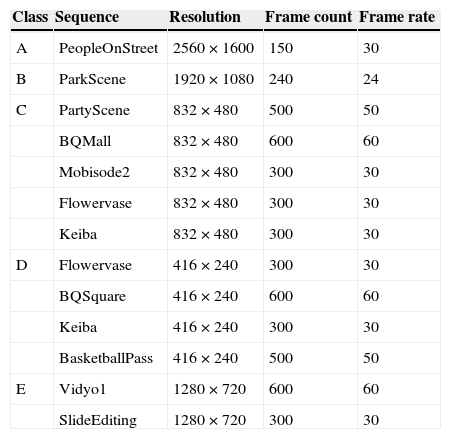
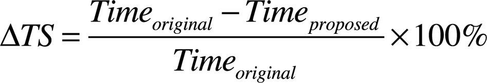
The proposed feature-based CU partition algorithm has been implemented in the test model HM10.1 to conduct related experiments for evaluating its performance. The experiment platform is equipped with Microsoft Windows 7 Professional Service Pack 1 32-bit O/S, Intel^® Core^® i7-2600 3.4 GHz CPU and 4 GB RAM. Table 4 describes the video sequences that were used in the experiments. There are thirteen sequences classified into five classes of resolution used for the test. The experimental HEVC parameters are conditioned with main profile, intra only coding structure and QPs varying at 24, 28, 32 and 36. The coding efficiency is measured by BD-Rate, BD-PSNR (Bjontegaard, 2001) and time-savings. The time-savings () is defined as:

Table 4.

Experiment sequence.

Class	Sequence	Resolution	Frame count	Frame rate
A	PeopleOnStreet	2560 × 1600	150	30
B	ParkScene	1920 × 1080	240	24
C	PartyScene	832 × 480	500	50
	BQMall	832 × 480	600	60
	Mobisode2	832 × 480	300	30
	Flowervase	832 × 480	300	30
	Keiba	832 × 480	300	30
D	Flowervase	416 × 240	300	30
	BQSquare	416 × 240	600	60
	Keiba	416 × 240	300	30
	BasketballPass	416 × 240	500	50
E	Vidyo1	1280 × 720	600	60
	SlideEditing	1280 × 720	300	30

Figure 15 demonstrates the image frames of the test sequences. The main properties of each video are described briefly in the following. The ‘PeopleOnStreet’ sequence is high definition video sequence, which contains higher complex image structure. The ‘ParkScene’ sequence shows smooth, variation structure and object moving characteristics. The ‘PartyScene’ sequence has zooming effects, object moving, complex structure and lighting noise. The ‘BQMall’ sequence renders variation image structure, and sometimes appears objects close to the camera. The ‘Mobisode2’ sequence presents a very dark video with people entering an elevator carriage. It has suddenly brighten, darken and change scenes. The ‘Flowervase’ possesses the screen zooming with brightness slowly changing from dark to bright. The ‘Keiba’ sequence is kind of fast moving sequence. Sometimes, the moving objects are occluded with each other at the video scenes. The ‘BQSquare’ sequence presents some complex image structure, screen zooming and slowly moving objects. The ‘BasketballPass’ contains suddenly fast moving objects. The ‘Vidyo1’ possesses a static background and a part of slowly moving region in the scene. Unlike the other sequences, the ‘SlideEditing’ sequence is a computer screen video with pretty fine-grained and high constrast content.

Fig. 15.

Experiment sequence video. A: PartyScene. B: BQMall. C: Mobisode2. D: Flowervase. E: Keiba. F: BQSquare. G: BasketballPass. H: Vidyo1. I: SlideEditing. J: PeopleOnStreet. K: ParkScene.

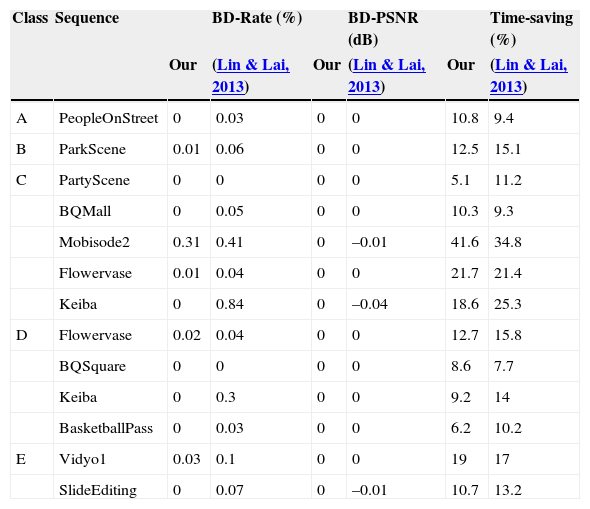
Table 5 shows the results by the proposed algorihtm and the method by Lin and Lai (2013). As revealed by the results, the proposed algorithm can provide time-savings ranging from 5.1% to 41.6% with respect to the test mode HM10.1. With more specifics to the case for the ‘Mobisode2’ sequence in class C, the proposed algorithm and the method by Lin and Lai (2013) exhibit time-savings up to 41.6% and 34.8%, respectively. At the same time, they also undego about 0.31% and 0.41% BD-Rate increase when compared to other sequences. This is because the edge features are not so strong that the proposed algorithm would not make more accurate classifcation of partition classes for CTBs in this sequence. With that, the proposed algorithm is still able to offer 6.8% more time-saving than that by Lin and Lai (2013) under a less BD-Rate about 0.1%.

Table 5.

Results for comparison with Lin and Lai (2013).

Class	Sequence		BD-Rate (%)		BD-PSNR (dB)		Time-saving (%)
		Our	(Lin & Lai, 2013)	Our	(Lin & Lai, 2013)	Our	(Lin & Lai, 2013)
A	PeopleOnStreet	0	0.03	0	0	10.8	9.4
B	ParkScene	0.01	0.06	0	0	12.5	15.1
C	PartyScene	0	0	0	0	5.1	11.2
	BQMall	0	0.05	0	0	10.3	9.3
	Mobisode2	0.31	0.41	0	–0.01	41.6	34.8
	Flowervase	0.01	0.04	0	0	21.7	21.4
	Keiba	0	0.84	0	–0.04	18.6	25.3
D	Flowervase	0.02	0.04	0	0	12.7	15.8
	BQSquare	0	0	0	0	8.6	7.7
	Keiba	0	0.3	0	0	9.2	14
	BasketballPass	0	0.03	0	0	6.2	10.2
E	Vidyo1	0.03	0.1	0	0	19	17
	SlideEditing	0	0.07	0	–0.01	10.7	13.2

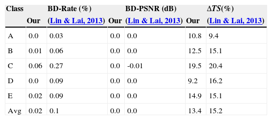
Table 6 compares the proposed method with our previously developed method (Lin & Lai, 2013) on the summary results of all the considered sequences. The proposed method would slightly increase BD-Rate by 0.02% and maintain PSNR-Y 0 dB on average. However, the time-savings about 13.4% could be achieved on average. While the previously proposed method (Lin & Lai, 2013) shows an increase of average time-saving up to 1.8% when compared to the proposed method, it also suffers an addition of BD-Rate by 0.09% in relative to that of the propose algorithm.

Table 6.

Summary of experiment results.

Class		BD-Rate (%)		BD-PSNR (dB)		ΔTS(%)
	Our	(Lin & Lai, 2013)	Our	(Lin & Lai, 2013)	Our	(Lin & Lai, 2013)
A	0.0	0.03	0.0	0.0	10.8	9.4
B	0.01	0.06	0.0	0.0	12.5	15.1
C	0.06	0.27	0.0	-0.01	19.5	20.4
D	0.0	0.09	0.0	0.0	9.2	16.2
E	0.02	0.09	0.0	0.0	14.9	15.1
Avg	0.02	0.1	0.0	0.0	13.4	15.2

Figure 16 depicts the time-savings curves for the three sequences with which the proposed algorithm can behave better than the method by Lin and Lai (2013). On the other hand, Figure 17 shows the time-savings for the other sequences. For the cases shown in Fig. 17, the proposed algorithm is inferior to the method (Lin & Lai, 2013). The reason for this phenomenon is that the smooth region in these sequences occupies a higher proportion of most video frames in them. For smooth region, the proposed method selects class A to partition the CTBs, which requires partitioning to depth 2, while the method by Lin and Lai (2013) always partitions with depth 0 and 1. For example, with the co-located smooth region shown in Figure 18A, one CTB is partitioned into a quad-tree with depth 1 (Fig. 18B) by the method (Lin & Lai, 2013). For another smooth CTB shown in Figure 19A, the proposed algorithm classifies the CTB to class A and outputs a partitioned quad-tree with depth of 2, as that shown in Figure 19B. In this case, the proposed method requires more computation for partition depth from 0 to 2.

Fig. 16.

Time-savings in BQMall_832x480 (A), Vidyo1_1280x720 (B), and PeopleOnStreet_2560x1600 (C).

Fig. 17.

Time-savings for Keiba_416x240 (A), PartyScene_832x480 (B), ParkScene_1920x1080 (C), and SlideEditing_1280x720 (D).

Fig. 18.

Smooth region for Lin and Lai (2013) method. A: co-located block. B: quad-tree partition of current CTB.

Fig. 19.

Smooth region for proposed method. A: current CTB. B: quad-tree partition of current CTB.

However, in the case for ‘BQMall’, ‘Vidyo1’ and ‘PeopleOnStreet’ videos, the proposed method can obtain a better time-savings. This is because these sequences have rich complex variations of image structure. For more complex variation structure, the method by Lin and Lai (2013) is difficult to obtain the best time-saving compared to the proposed method. For example, the Figures 20 and 21 show partition cases for complex CTB by the method (Lin & Lai, 2013) and the proposed method, respectively. In Figure 20, the method (Lin & Lai, 2013) needs to process depth levels from 0 to 3 based on the information from the co-located CTB. But the proposed method shown in Figure 21 requires only processing from depth 1 to 3. It skips depth 0 to process. Figure 22 shows the BD-BitRate between the proposed method and the method (Lin & Lai, 2013). It can be seen that the proposed method has lower BD-BiteRate, in comparison with that by Lin and Lai (2013) on each sequence. Results in Figures 22C and E reveal that the proposed algorithm obtains the best compression performance. The reason behind the fact is that there are a lot of highly complex structures existed in the frames of the sequence. For the more detailed structure, it uses the smaller blocks as the good partition to maintain the video quailty and keep the compression ratio. Otherwise, it makes a great deal of large residual signal when employing the larger blocks to partition. The previous method (Lin & Lai, 2013) does not consider the image variation structure; therefore, it obtains the inferior partition for the complex variation structure region.

Fig. 20.

Complex region by Lin and Lai (2013) method. A: co-located block. B: quad-tree partition of current CTB.

Fig. 21.

Complex region by proposed method. A: current CTB. B: quad-tree partition of current CTB.

Fig. 22.

BD-Rate. A: Keiba. B: FlowerVase. C: BQMall. D: Mobisode2. E: SlideEditing. F: Vidyo1. G: ParkScene. H: PeopleOnStreet.

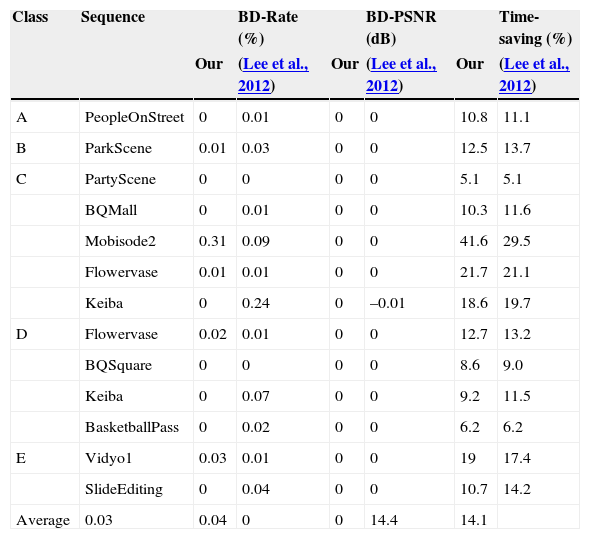
Consider another method (Lee et al., 2012) for comparison. This method uses the co-located CTB information in the previous encoded frames as the basic classifying criterion. Table 7 demonstrates the comparison of results between the proposed method and the method (Lee et al., 2012), where the average time-savings and BD-Rate do not have significant difference between them.

Table 7.

Results for comparison with Lee et al. (2012).

Class	Sequence		BD-Rate (%)		BD-PSNR (dB)		Time-saving (%)
		Our	(Lee et al., 2012)	Our	(Lee et al., 2012)	Our	(Lee et al., 2012)
A	PeopleOnStreet	0	0.01	0	0	10.8	11.1
B	ParkScene	0.01	0.03	0	0	12.5	13.7
C	PartyScene	0	0	0	0	5.1	5.1
	BQMall	0	0.01	0	0	10.3	11.6
	Mobisode2	0.31	0.09	0	0	41.6	29.5
	Flowervase	0.01	0.01	0	0	21.7	21.1
	Keiba	0	0.24	0	–0.01	18.6	19.7
D	Flowervase	0.02	0.01	0	0	12.7	13.2
	BQSquare	0	0	0	0	8.6	9.0
	Keiba	0	0.07	0	0	9.2	11.5
	BasketballPass	0	0.02	0	0	6.2	6.2
E	Vidyo1	0.03	0.01	0	0	19	17.4
	SlideEditing	0	0.04	0	0	10.7	14.2
Average	0.03	0.04	0	0	14.4	14.1

To show more detail information, Figure 23 illustrates the time-savings performance with varying QP values for some special sequences with complex image structure. As can be seen from the figures, the proposed method obtains comparable or even better than the method (Lee et al., 2012). The method (Lee et al., 2012) requires partitioning with depth levels 0 to 3 for the complex CTB in these sequences, while our proposed method needs one less depth level for the same CTB. Figure 24 shows the inferior cases of time-saving when compared with the method by Lee et al. (2012). Because these sequences have smooth region and the compared method encodes with depth level from 0 to 1, which is less than the proposed method, the proposed method offers inferior time-savings performance for the same CTBs.

Fig. 23.

Time-savings. A: BasketballPass. B: PartyScene. C: PeopleOnStreet.

Fig. 24.

Time-savings. A: Keiba. B: BQMall. C: ParkScene.

Figure 25 shows the BD-Rate comparison with the Lee's method (Lee et al., 2012) for the sequences with fast moving objects. The proposed method makes the better compression ratio in these considered sequences. This is because the proposed method adopts the edge features as the classification criterion, thus the edge features of details structure in CTBs actually reflect the visual content and give a good estimation of partition sizes.

Fig. 25.

BD-rate in Keiba sequence.

Figure 26 compares the BD-Rates for the sequence with insignificant edge features. In this case, the proposed algorithm does not has better ability to make accurate prediction of partition size. But Lee's method (Lee et al., 2012) uses the correlation between frames to obtain the prediction. The sequence is highly correlated, so the prediction of parition size is more accurate.

Fig. 26.

BD-rate in Mobisode2 sequence.

5

Conclusions

This paper proposes a feature-based CU partition algorithm for CTBs in HEVC intra coding. The algorithm uses the image feature defined as the edge density to classify the set of depth levels and reduce the computation burden for partition each incoming CTB. Experiment results have shown that the proposed algorithm could offer up to 41.6% of time-savings in HEVC intra coding at the expense of BD-Rate increase of 0.31% and extremely low BD-PSNR reduction.The performace of the proposed algorithm depends on the amount of prominent edge features in the video frames. The more prominent image features the video frames have the more time-savings the algorithm can obtain. When compared to the previous methods (Lee et al., 2012; Lin & Lai, 2013), the BD-Rate is significantly decreased and the time-savings are very comparable for most natural video sequences. The proposed method has shown a promising performance for reducing the computation complexity of HEVC encoding procedure by dealing with the meaningful features of content in CTBs. In the future, a hybrid approach that can adaptively react to the smooth and complex CTBs is worthy to receive much attention from the reseach domain for further development.

Acknowledgment

This research is supported in part by the Ministry of Science and Technology, Taiwan, under the grant No. NSC 102-2221-E-105-003-MY2.