H2 control of a one-quarter semi-active ground vehicle suspension

Abstract

Magneto-rheological (MR) dampers are effective solutions in improving vehicle stability and passenger comfort. However, handling these dampers implies a strong effort in modeling and control. This research proposes an H₂ controller, based on a Takagi–Sugeno (T–S) fuzzy model, for a two-degrees-of-freedom (2-DOF) one-quarter vehicle semi-active suspension with an MR damper; a system with important applications in automotive industry. Regarding performance criteria (in frequency domain) handled herein, the developed controller considerably improves the passive suspension's efficiency. Moreover, nonlinear actuator dynamics usually avoided in reported work, is included in controller's synthesis; improving the relevance of research outcomes because the controller is synthesized from a closer-to-reality suspension model. Going further, outcomes of this research are compared (based on frequency domain performance criteria and a common time domain test) with reported work to highlight the outstanding results. H₂ controller is given in terms of quadratic Lyapunov stability theory and carried out by means of Linear Matrix Inequalities (LMI), and the command signal is applied via the Parallel Distributed Compensation (PDC) approach. A case of study, with real data, is developed and simulation work supports the results. The methodology applied herein can be extended to include other vehicle suspension's dynamics towards a general chassis control.

1

Introduction

Suspension system in a vehicle has the objective of absorbing road disturbances, while keeping the tires in contact with the road surface (Gillespie, 1992; Milliken & Milliken, 1995; Wong, 2001). At the same time it improves passenger comfort and vehicle stability in a certain level. Traditional, commercial oriented suspensions are passive, and are permanently designed for comfort or stability purposes. The problem consists in the trade-off relation between comfort and stability.

Last decade has seen technological advances in fabrication, modeling and control of special materials. As research on these materials achieved more and more results, generations of economically viable vehicle suspensions became available. Modern technology includes state-of-the-art vehicle shock absorbers that modify their damping force in real-time. These types of suspensions are commonly known as intelligent suspensions (Pauwelussen & Pacejka, 1995).

As part of intelligent semi-active suspensions, magneto-rheological dampers (MR) are one of the most applied and explored options due to their low power consumption and safety (Spencer Jr., Dyke, Sain, & Carlson, 1997). Strong efforts in recent time have been oriented towards alternative actuators that can compete with MR dampers, i.e. Gysen, Janssen, Paulides, and Lomonova (2009) merged a brushless tubular permanent-magnet actuator with a passive spring, whereas Kruczek, Stríbrský, Hyniová, and Hlinovský (2008) employed a linear motor as the actuator. Moreover, Pan and Hao (2011) inserted an air spring actuator to improve passenger comfort via LQG control (Green & Limebeer, 1995). Despite of the latest approaches, MR dampers remain the most referred actuators in intelligent suspension systems (Abu-Ein, Fayyad, Momani, Al-Alawin, & Momani, 2010).

Insertion of MR dampers into vehicle suspensions can considerably increase ride comfort and vehicle stability. However, the system's complexity is enlarged because of the hard nonlinearities phenomenon inherent in damper's composition (Worden & Tomlinson, 2001). As a consequence, modeling and control strategies for semi-active suspensions are two principal areas where automotive investigation has been concentrated.

Reported state-of-the-art for one-quarter vehicle suspensions is extensive and diverse. A part of reported work has focused on a 2-DOF differential equations model restricted to vertical dynamics. For instance, Sammier, Sename, and Dugard (2003) included performance criteria in frequency and time domains, and calculated an H_∞ controller (Zhou, Doyle, & Glover, 1996) without including the actuators dynamics in controller's computation. Moreover, Poussot-Vassal et al. (2008) achieved a robust suspension system through linear parameter varying (LPV) theory. Recently, Zapateiro, Pozo, Karimi, and Luo (2012) developed two control approaches: H_∞ control and quantitative feedback theory (QFT). Results were presented in frequency and time domains. Another up-to-date work is Krause and Kaspersky (2014), where frequency domain results were presented to compare suspension's performance. This study carried out a controller formulation that took into account an MR damper modeled via Bouc–Wen.

Another branch of active suspensions has followed H₂ or LQG (Linear Quadratic Gaussian) approaches. The work presented in De Jagger (1991), Shi-hong and Hui-hui (2011), Turkay and Akcay (2007), Chen, Zhou, Liu, and Yao (2011) proposed an LQG or LQG/LQI (Linear Quadratic Integral) control aimed to ride comfort improvement in a one quarter vehicle suspension. However, results were limited to time domain. An opportunity area to these contributions could be the incorporation of actuator dynamics in control synthesis formulation. As far as authors are concerned, Akbari, Koch, Pellegrini, Spirk, and Lohmann (2010) reported an outstanding multi-objective H_∞/LQG control for a one-quarter 2-DOF vehicle suspension, including the nonlinear actuator's dynamics in control synthesis, as well performance criteria; however, results are restricted to time domain.

By extending suspension system to a half-vehicle, Zhang, Xia, Qin, and Zhang (2010) also applied the LQG approach to improve ride comfort and handling stability (chassis and pitch angle accelerations, as well as vertical displacements of wheels). Furthermore, Xiao, Chen, Zhou, and Zu (2009) presented a full-vehicle suspension control via an LQG control that applied adaptive fuzzy logic. Results in time domain warrant: suspension handling, vehicle stability and passenger comfort. However, the research did not include actuator dynamics neither frequency domain tests. These are opportunity areas considered in the present work.

Recently, Cao, Li, and Liu (2010) reported a fuzzy controller for a one-half semi-active suspension modeled via T-S approach (Takagi & Sugeno, 1985), whereas El Messoussi, Pages, and El Hajjaji (2007) went further and developed a T–S fuzzy model and control for the four wheels vehicle model, but in both cases, MR damper dynamics were left aside and no performance criteria in frequency domain were included. Thus, the intention of this research is to perform a control analysis that includes actuator's nonlinear dynamics. The baseline herein considers the suspension model and stability analysis reported in Félix-Herrán, Mehdi, Soto, Rodríguez-Ortiz, and Ramírez-Mendoza (2010) and calculates an H₂ controller to comply with a set of relevant performance criteria. As benchmark tests, results are compared with previous reported work (Do, Sename, & Dugard, 2010; Du & Zhang, 2009; Poussot-Vassal et al., 2008; Sammier et al., 2003) that applied alike testing conditions and performance indexes.

This article is organized as follows: Section 2 presents the semi-active one-quarter vehicle system, and the T–S fuzzy modeling. Section 3 includes the H₂ control synthesis via LMIs approach, whereas Section 4 lists and describes frequency performance criteria. Section 5 presents a case of study based on real vehicle suspension and MR damper data. In Section 6, a comparison with reported outcomes is implemented. Last section concludes the investigation and includes further research possibilities.

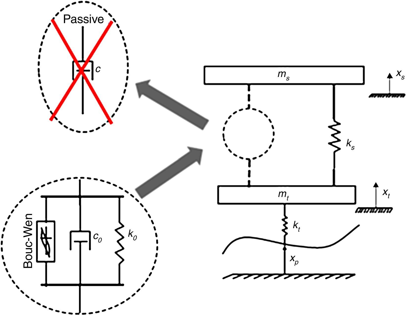
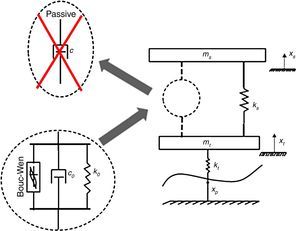
2

Semi-active fuzzy modeling

This research considers the T–S fuzzy model for a one-quarter-vehicle suspension model with an MR damper, where the damper is modeled via the Bouc–Wen approach (Spencer Jr. et al., 1997). Referred suspension system is portrayed in Figure 1, a well-known passive representation widely accepted for vehicle suspension analysis.

Figure 1.

One-quarter vehicle suspension model with a MR damper (represented by the Bouc–Wen model).

In Figure 1, m_s stands for one quarter of the suspended mass; m_t represents the non-suspended mass (tire, damper, spring, etc.), x_s and x_t are the masses’ displacements, and x_p represents the road profile, described by a disturbance in the form of x_p = Asin(ωt). k_t is the tire stiffness, whereas k_s is the spring between the tire and the chassis. Finally, parameter c represents a passive damping coefficient.

In accordance with Figure 1, passive damper is changed with a magnetorheological damper. Hence, parameter c is replaced with a MR damper (composed by c₀, k₀, and hysteresis) modeled via the Bouc–Wen approach (Sireteanu, Stancioiu, & Stammers, 2001; Spencer Jr. et al., 1997). The suspension model becomes nonlinear because of: hysteresis, saturation due to the masses, and viscoplasticity characteristics of the fluid inside the damper (Worden & Tomlinson, 2001). k₀ and c₀ stand for large velocities stiffness and viscous damping, respectively. Resulting semi-active suspension is represented through T–S fuzzy approach.

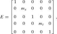
Eqs. (1) and (2), include an evolutionary variable Bouc–Wen Z_BW related to the MR damper's hysteresis phenomenon (Spencer Jr. et al., 1997). Z_BW depends on displacement time history, as in Eq. (3). Furthermore, parameters: γ, β, δ and n = 2, are determined by the form of hysteresis behavior in the MR damper.

Presented in Takagi and Sugeno (1985), a T–S fuzzy model is a set of linear subsystems interconnected via fuzzy membership functions, where each subsystem has the form of IF… THEN rules, with a premise and a consequent. Following the T–S approach in Tanaka, Ikeda, and Wang (1996), as well as Tanaka and Wang (2001), the system reported in Félix-Herrán et al. (2010) can be put together in a descriptor form, as performed in Félix-Herrán, Mehdi, Rodríguez-Ortiz, Soto, and Ramírez-Mendoza (2012). One advantage of a descriptor representation is its capability to describe a more general type of systems than conventional state-space models (Luenberger, 1977). More recently, Tanaka, Ohtake, and Wang (2007) exposed other advantages of descriptor systems related to fuzzy control systems design. The Takagi–Sugeno fuzzy model representation considered for the present research is as follows:

In Eq. (4), E is the matrix of masses; it is invertible and diagonal (a symmetric matrix) (Verghese, Levy, & Kailath, 1981). A_i are the state matrices, B_ui are input vectors related to the command signal, whereas B_w is the input vector that connects disturbances with the rest of the system. x(t) is the state vector, u(t) is the command input and x_p(t) represents the disturbance input from the road profile. h_i functions contain the suitable combinations of all defined membership functions, according to T–S approach in Tanaka et al. (1996), and Tanaka and Wang (2001). It is important to accentuate that the nonlinear characteristics of the T–S fuzzy modeling are enclosed in the appropriate definition of membership and h_i functions as reported in Félix-Herrán et al. (2010), and Félix-Herrán et al. (2012). The complete modeling is a well-suited representation of Eqs. (1)–(3), where the whole T–S fuzzy design in Eq. (4) is nonlinear (Tanaka & Wang, 2001).

This research considers the model reported in Félix-Herrán et al. (2010), that has four linear subsystems interconnected by fuzzy membership functions, hence N = 4. State vector x(t) consists of five state variables (x₁ is the sprung mass displacement, x₂ represents the sprung mass velocity, x₃ refers to the unsprung mass displacement, x₄ is the tire mass velocity, and x₅ refers to the theoretical internal variable Z_BW. Matrices A_i and E have dimensions [5×5] due to the five state variables.

A_i = A + Γ_i with

where Γ_I is defined as follows: Γ₁ = Γ₃ = e^Tb_maxe; Γ₂ = Γ₄ = e^Tb_mine, with e=[00001]. Applied current i into the actuator affects the internal MR dampers’ characteristics with the variation of parameters: c₀, k₀, and α, as in Spencer Jr. et al. (1997).

In Eqs. (7)–(9), c_0a, c_0b, k_0a, k_0b, α_a and α_b are the parameters that compose the linear relation between current i and parameters c₀, k₀, and α, respectively, as fully explained in Spencer Jr. et al. (1997).

T–S fuzzy modelling applied in this research considers a system with two nonlinearities and each nonlinear term is bounded. a_max and a_min represent the maximum and minimum values of one nonlinearity and the same rationale applies for the second nonlinearity (b_max and b_min).

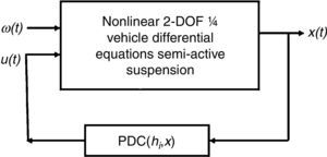
T–S model in Eq. (4) is valid if conditions in Eqs. (13) and (14) hold. These restrictions are related to affine h_i functions, as fully explained in Tanaka et al. (1996), and Tanaka and Wang (2001).

The next step is to work on the controller formulation. An H₂ control strategy is developed for the semi-active suspension in Figure 1.

3

Controller synthesis

In this section, the work is divided in three stages: control formulation, a mathematical approach to deal with ill-conditioned matrices, and the suspension system in practice.

3.1

H₂ control

From Eq. (4), each linear subsystem of the T–S model can be represented by

In Eqs. (15) and (16), C_z is the output vector, D_u and D_w are the feedforward matrices related to command signal and disturbances, respectively. These matrices will be defined in Section 5 for the experimental example. x(t) is the state vector, u(t) is the command input, and w(t) is the disturbance signal that comes from the road profile. z(t) is the controlled output vector that complies with H₂ formulation. System's matrices in Eq. (15) were explained just after Eq. (4).

The H₂ approach is based on the H₂ norm (Zhou et al., 1996), defined below

In Eq. (17), the left part represents the largest singular value of transfer function G_zw, which is the (controlled output z/input disturbance w) relation along all the frequency range ω of finite and bounded energy (Scherer & Weiland, 2005). In the right part, G_zw*(jω) stands for the complex conjugate transpose of G_zw(jω). Hence, H₂ controller pursues to keep the G_zw norm small (inferior to an arbitrary value) in the presence of disturbance signals, w(t). Output vector z(t) must contain the variables mentioned in the performance criteria (Levine, 2000).

Considering the system defined in Eqs. (15) and (16), Boyd, El Ghaoui, Feron, and Balakrishnan (1994) present an H₂ problem formulation for controller synthesis. If the pair (A_i, B_u) is at least stabilizable, the pair (C_z, A_i) is at minimum detectable, and matrices D_u and D_w are both zero, a prescribed H₂ performance γ > 0 designs a controller that seeks to keep the regulated (controlled output z(t)/input disturbance w(t)) relation below some prescribed value.

To synthesize the controller gains, the formulation is expressed as a set of Linear Matrix Inequalities (LMI) (Boyd et al., 1994; VanAntwerp & Braatz, 2000). To calculate a control law in the form of a static state feedback controller u(t) = Kx(t) that complies with a norm H₂ smaller or equal than γ, two matrices P and W must be computed and they have to meet a set of LMIs. The following formulation determines a controller that stabilizes the system and simultaneously guarantees a disturbance rejection of level γ > 0.

In Eq. (18), P represents the Lyapunov matrix related to quadratic stability (31).

Linear Matrix Inequalities in Eqs. (18) and (19) must hold for ∀(i, j) = 1, 2, …, N, where N is the number of subsystems.

In Eqs. (18)–(22), W and P are positive-definite symmetric matrices. Moreover, and auxiliary variable Yj is defined.

Eq. (23) relates the auxiliary matrix Y_j in Eqs. (18) and (19). In addition, Y_j allows another adjustable parameter in the controller computation. The set of LMIs in Eqs. (18)–(22) conform the well-known LMI feasibility problem (Boyd & Vandenberghe, 2004) for computing the set of K_j.

Due to controller's fuzzy nature, the command signal is computed in accordance with the Parallel Distributed Compensator (PDC) approach (Tanaka et al., 1996; Tanaka & Wang, 2001); a design technique that fuzzy blends the action of each local controller gain K_j to generate u(t).

In Eqs. (18), (19), (23), and (24), i and j = 1, 2,…, N, where N represents the number of subsystems in the T–S fuzzy model.

3.2

State-space transformation

It is well known that a state space model has many equivalent representations through the original system multiplied by a transformation matrix T (Green & Limebeer, 1995; Williams II & Lawrence, 2007). Some representations are more suitable for controller synthesis that others (Ogata, 2000). Even though system's matrices change, the characteristic polynomial and eigenvalues of matrix A do not change, hence, the initial and transformed representations are equivalent. Albeit eigenvectors are different between the original and transformed systems, they are related via the T matrix.

One advantage of a transformation matrix is that it could reduce ill-conditioning conditions. In some applications, e.g., automotive suspension control, systems formulation contains elements around the unity whereas other parameters are thousands of times larger or smaller; hence, the generated system matrices present an ill-conditioning behavior. When the inverse of these matrices is required, the inversion method presents converging and therefore, controller synthesis computation could fail. A possible solution is to apply the transformation procedure to obtain an alternative state-space realization that will not present the ill-conditioning problem.

The transformation matrix approach is employed herein because partial results during the research generated ill-conditioned matrices coming from ill-conditioned data. It is straightforward to detect these types of matrices (A_i) because semi-active suspension parameters are different among them in the order of thousands of units. To solve this problem, this research applies equivalent state space realizations based on a transformation matrix. With the system in Eqs. (15) and (16), a transformation matrix T is declared in such a way that

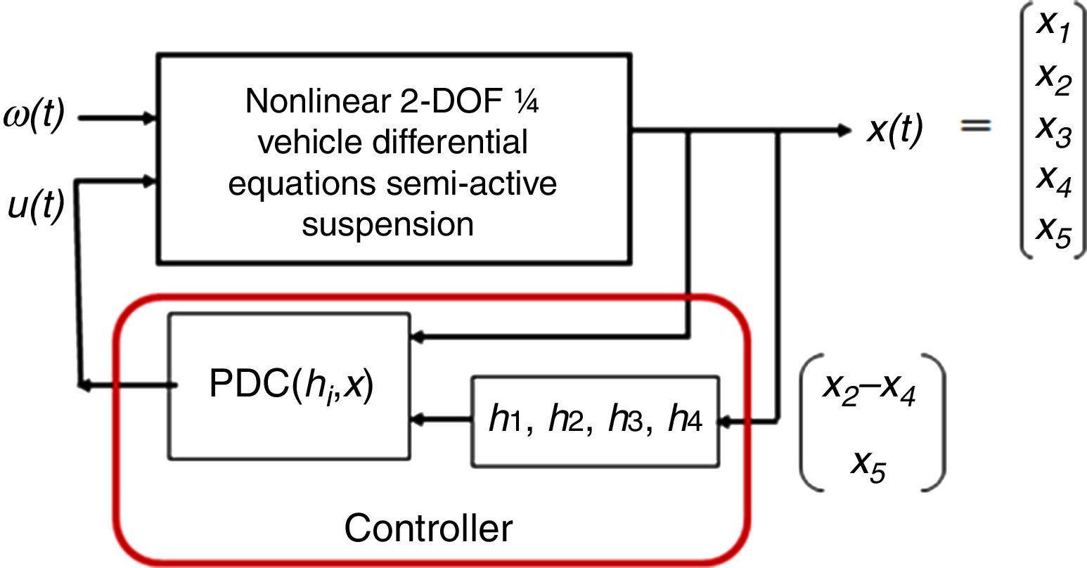
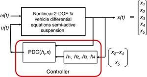
The transformed system is

The system in Eqs. (26) and (27) is equivalent to the one defined in Eqs. (15) and (16). Besides, if

Eq. (26) can be rewritten as follows

In Eq. (29), a modified gain is calculated to work for a modified vector x_T(t). However, it is important to consider that after the controller is been computed, T–S fuzzy model is left aside and the controller is applied to the original nonlinear differential equations system, ergo controller gain has to be returned to the original system's coordinates.

Returning to LMI conditions in Eqs. (18)–(24), the feasibility problem, Boyd and Vandenberghe (2004) has to be applied for the set of LMIs; therefore, a controller gain that meets LMI formulation in Eqs. (18)–(22), has to be obtained.

3.3

The closed-loop semi-active suspension in practice

The closed-loop semi-active suspension system in practice is depicted in Figure 2. After the controller is computed and the T–S model is dropped, only the controller gains (combined in the form of a PDC), along with h_i(t) nonlinear functions are preserved and applied to build the closed-loop structure. Tests are run with the original nonlinear differential equations model, as reported in Félix-Herrán et al. (2010). For the present case of study, state vector x(t) is considered completely measurable, except the theoretical variable Z_BW estimated from the other variables in x(t). Results are presented as describing functions, which are Bode diagrams for nonlinear systems (Slotine & Li, 1991).

Figure 2.

Semi-active suspension system. The feedback vector is the input to the PDC.

4

Performance criteria

Few reported articles on automotive suspensions include clear performance criteria indexes related to frequency and time domains. Research work herein refers to the criteria in Wong (2001), Sammier et al. (2003), and Poussot-Vassal et al. (2008).

• ∘

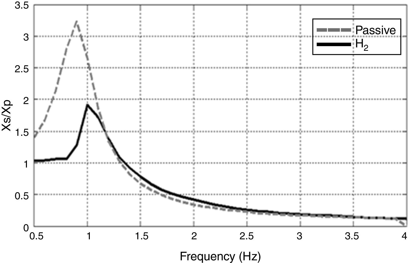
  Ride comfort in low frequencies (0–4 Hz). Limit the relation (chassis displacement/road profile), i.e. (x_s/x_p) to be less than 2. In general, the idea is to reduce the resonance peak around the sprung mass resonance frequency (approx. 1.1 Hz for an average city vehicle). Disturbance signal is represented with a sinusoidal signal of the form x_p = 0.015 sin(ωt) (amplitude in meters).

• ∘

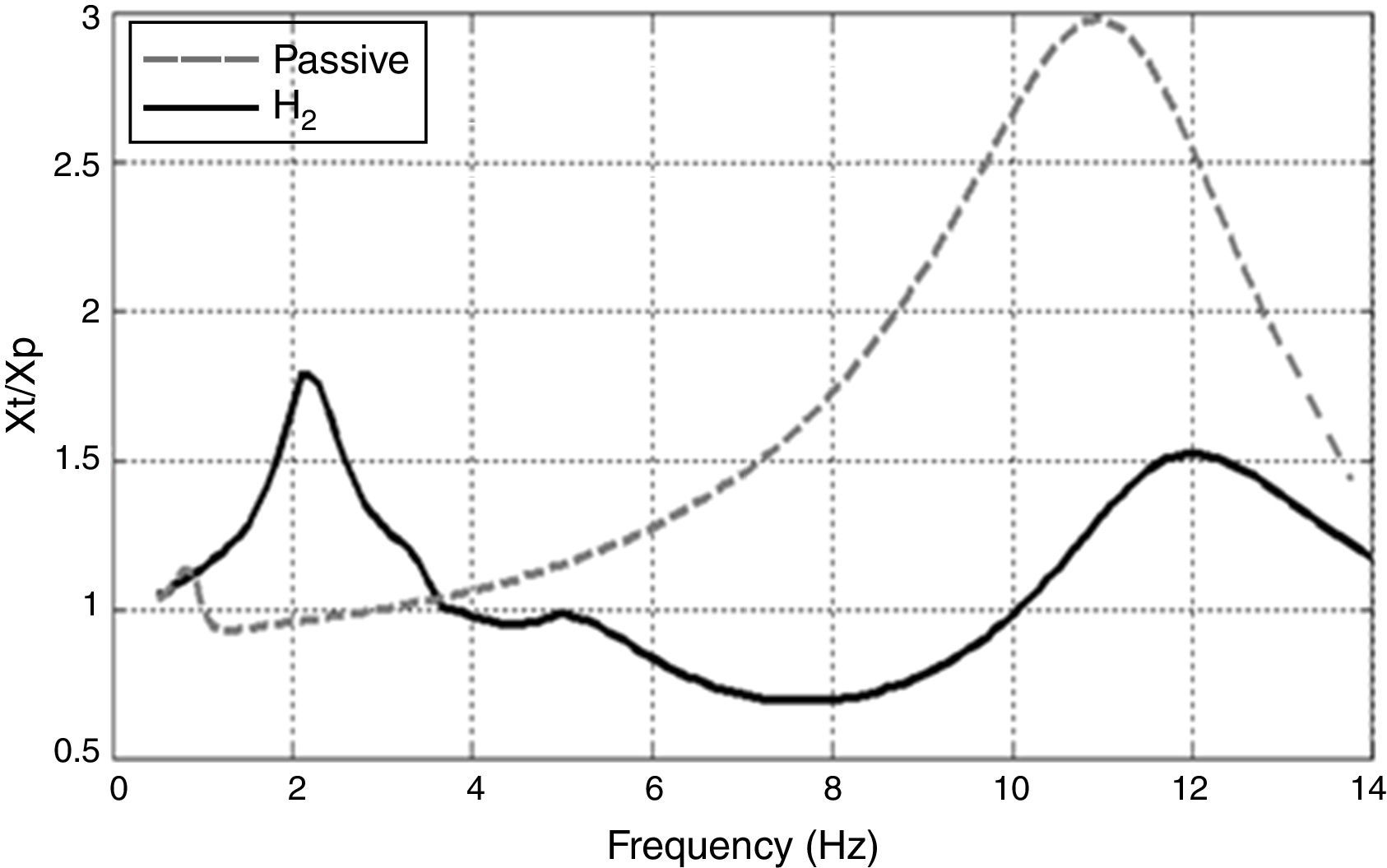
  Road holding (vehicle stability) (0–15 Hz). The same as in ride comfort but with the relation (tire displacement/road profile), i.e. (x_t/x_p). The objective is to reduce the unsprung mass resonant peak around 10 Hz (average city vehicle). Disturbance signal is represented with a sinusoidal signal with the following form x_p = 0.001 sin(ωt) (amplitude in meters).

• ∘

  Comfort at high frequencies (4–30 Hz). Response of the chassis acceleration (x¨s) to the excitation from the ground. Keep the root mean square acceleration (rms) of the chassis below some boundaries limits as reported in Wong (2001), to ensure a passenger comfort condition during 8 h. Disturbance signal for this test is the same as for road holding.

• ∘

  Suspension travel (x_s–x_t) within physical limits (0–4 Hz). To increase damper's life cycle, and avoid non-modeled dynamics when the suspension limits (±2.5 cm for specific MR damper mentioned in the case of study) are reached. Disturbance signal for this test is the same as for ride comfort in low frequencies.

• ∘

  Time domain (road bump test). Despite there is no specific time domain criteria indexes for automotive suspensions, the goal is to reduce in a considerably amount, the overshoot and settling time of: chassis displacement, tire displacement, chassis acceleration, and suspension deflection as well. For the latter variable, in addition of physical limits avoidance, the deviation from the reference position has to be as small as possible. This is the criterion used in literature (Karlsson, Dahleh, & Hrovat, 2001; Sammier et al., 2003; Slotine & Li, 1991).

5

Experimental example and results

This research considers the one-quarter suspension reported in Félix-Herrán et al. (2010), a system with two nonlinearities (Z₁ and Z₂) and according to T–S fuzzy modeling in Akbari et al. (2010), with four linear subsystems generated (N = 4) in Eq. (24). Subsystems are connected by four fuzzy membership functions (M₁, M₂, N₁, and N₂).

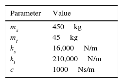
To support theoretical work, simulations were carried out in MATLAB-Simulink with numerical data from a real MR damper characterization (Sireteanu et al., 2001). In addition, suspension's values were taken from Félix-Herrán et al. (2012) and are listed in Table 1.

Table 1.

One-quarter vehicle suspension parameters.

Parameter	Value
ms	450 kg
mt	45 kg
ks	16,000 N/m
kt	210,000 N/m
c	1000 Ns/m

It is important to emphasize that Bouc–Wen parameters are difficult to obtain because a nonlinear identification process is demanded for calculating the parameters. There is previous work that highlights this complexity when phenomenological model structures are proposed (Ikhouane & Rodellar, 2007; Spencer Jr. et al., 1997). For simplicity, it is assumed that Bouc–Wen parameters remain constant over time (understanding this approach could be improved through nonlinear and adaptable identification schemes (Ljung, 1999). The aim of this research is not the Bouc–Wen modelling and parameters identification, but the application of an MR damper as part of a control strategy able to improve passenger comfort and vehicle stability.

From Sireteanu et al. (2001), Bouc–Wen model parameters are: γ = 1e⁶ m⁻², and δ = 15. Dynamic behavior of parameters: k₀, c₀, and α, are in Eqs. (31)–(33). These three damper's parameters were approximated by polynomial functions that depend on electrical current i. For this case of study, MR damper current's range is coerced into [0.2–1.75] A, as in Félix-Herrán et al. (2010).

There is a practical aspect to be considered in the T–S modeling. System's matrices are ill-conditioned, and some actions have to be performed to ameliorate this problem. To calculate the controller, the semi-active suspension is modeled via Takagi–Sugeno (T–S) approach, where two nonlinearities (Z₁ and Z₂) were identified. With actual parameters’ values, Z₂ has very large boundaries (Z_2min = approx. −1.0e³ and Z_2max = 0), and the magnitude of this range is related to the matrices’ conditioning.

From the experience on working with this type of suspension system (Félix-Herrán et al., 2012), and for controller synthesis purposes, equivalent MR damper data (γ_M, β_M and δ_M) can be heuristically calculated to decrease the nonlinearities boundaries. Hence, the new values were: γ_M = β_M = 1.0e⁵ m⁻², and δ_M = 1.37. To obtain the modified values, it was necessary to run a lot of simulations through empirical work before finding suitable values to generate smaller nonlinearity bounds and less ill-conditioned matrices.

When γ_M, β_M and δ_M replaced the original ones, and under the working conditions stated in this work, the error was kept below 1% when it was compared against the original system (this is for chassis displacement, the variable with the largest error). Regarding T–S fuzzy modeling, the nonlinearities’ boundaries were: a_max = 156, a_min = −166, b_max = 0, and b_min = −290. With these values, M₁, M₂, N₁, and N₂ were calculated. T–S validation, (33) was applied and the numerical values for matrices Eqs. (19)–(23) that represent the T–S model in Eq. (18), were obtained. The next step is to compute the H₂ controller.

For H₂ formulation in Eqs. (18)–(22), (chassis displacement/road profile) and (tire displacement/road profile) were included in the control formulation. The system variables affected by H₂ control were: sprung mass displacement x₁, and tire mass displacement x₃. Hence, matrices in Eq. (16) were numerically defined.

Following the approach reported in Félix-Herrán et al. (2012), (x˙s−x˙t) and Z_BW, represented the inputs for subsystems h_i(t) (for i = 1, …,4). State variables: x₂, x₄ and x₅, likewise h_i were considered part of the controller, u(t) was the command signal from the controller, whereas ω(t) was the road profile. The 2-DOF one-quarter vehicle nonlinear semi-active suspension model is the one reported in Félix-Herrán et al. (2010). The suspension system for this numerical example is portrayed in Figure 3.

Figure 3.

Semi-active suspension system. The feedback vector is the input to the PDC. hi(t) along and vector x(t) are the controller's inputs.

As explained in Section 3, closed-loop suspension system was checked for stabilizability and detectability before the LMIs were solved. For this example, each linear subsystem complied not only with the aforementioned properties, but also with controllability and observability conditions (Ogata, 2000).

Different state-space representations, as in Eq. (25) were tested. The modal state-space transformation contributed to generate the controller with the best results in frequency domain. This representation states that: if the system matrix A in Eq. (19), has no repeated eigenvalues, in the equivalent transformed realization the real eigenvalues and the complex conjugate eigenvalues (appear in 2-by-2 blocks) appear on the diagonal of the A matrix (Williams II & Lawrence, 2007).

A controller gain that complies with the LMI-H₂ controller formulation in Eqs. (18) and (22) was computed. The ill-conditioning problem (explained in Section 3.2) was improved by the modal state-space transformation, and the set of LMI were satisfied for γ = 60 (feasibility problem developed in MATLAB). Results summarized in Table 2.

Table 2.

Summary of frequency response results extracted from Figures 4 to 7.

Suspension	xs/xp gain	xt/xp gain	rms chassis acceleration. Does it meet comfort requirement?	max (xs–xt), in cm. Compliance with physical limits?
Passive	3.23	2.97	Yes	3.1 – no
Semi-active H2	1.91	1.78	Yes	1.2 – yes

5.1

Results in frequency domain

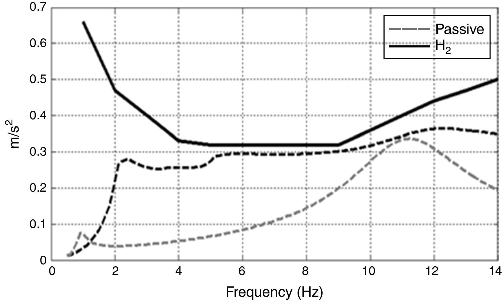
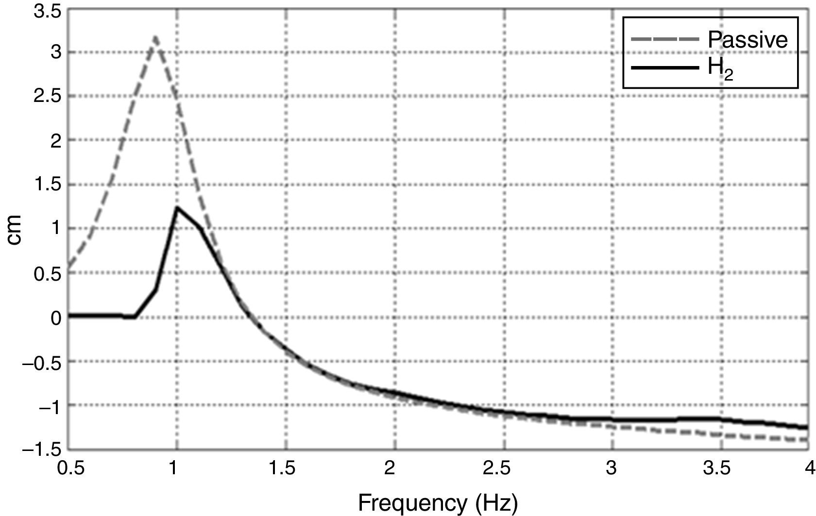
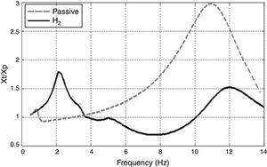
In general terms, suspension system with H₂ control complies with the four performance criteria presented in Section 4. Frequency domain tests, in Figures 4–7, support this statement.

Figure 4.

(x_s/x_p) relation for the passive and H₂ controlled suspensions.

Figure 5.

(x_t/x_p) relation for the passive and H₂ controlled suspensions.

Figure 6.

x¨ for the passive and H₂ controlled suspensions. Wide black line indicates the limits for chassis acceleration comfort (Wong, 2001).

Figure 7.

Suspension deflection (x_s–x_t) for the passive and H₂ controlled suspensions.

In Figures 4–7, simulation results provide evidence that proposed H₂ controller considerably enhances the passive suspension performance. In Figure 4, passive suspension fails to comply with an (x_s/x_p) maximum gain of 2, whereas H₂ controlled suspension keeps the maximum gain below 2. In Figure 5, the tire displacement resonant peak is shifted to smaller frequencies, but it is below the criterion gain value of 2. In Figure 6, chassis acceleration of the semi-active suspension has a higher rms value than its passive counterpart; however, it is kept below the comfort boundary limit (the wide black line indicates a passenger's comfort limit. If the root mean square acceleration (rms) of the chassis is below the line, a comfort situation will be maintained until for 8 h (Wong, 2001). In Figure 7, passive suspension reaches the damper's physical limits entering in a non-desired saturation state, whereas H₂ semi-active suspension has a maximum suspension deflection of 1.3 cm.

For chassis acceleration and tire displacement, the working frequency is smaller than mentioned in the performance criteria. The idea is to focus around the maximum gain, hence the simulation considers the frequency range from 0 to 14 Hz. Results in Figures 5 and 6 concentrate on the frequency range of interest, i.e., where the peak values are found. For the testing conditions herein, chassis acceleration and tire deflection follow a descendent behavior beyond 13 Hz.

As presented in Table 2, the H₂ controller complies with the four frequency domain performance criteria. Its solution is optimal in the sense that meets all the requirements; although, it is not the best in all the indexes.

Under testing conditions and constraints stated herein, the semi-active suspension complies with all the frequency domain performance criteria. It is demonstrated that a passive suspension is not able to meet the requirements.

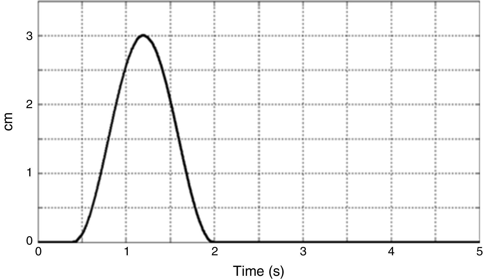
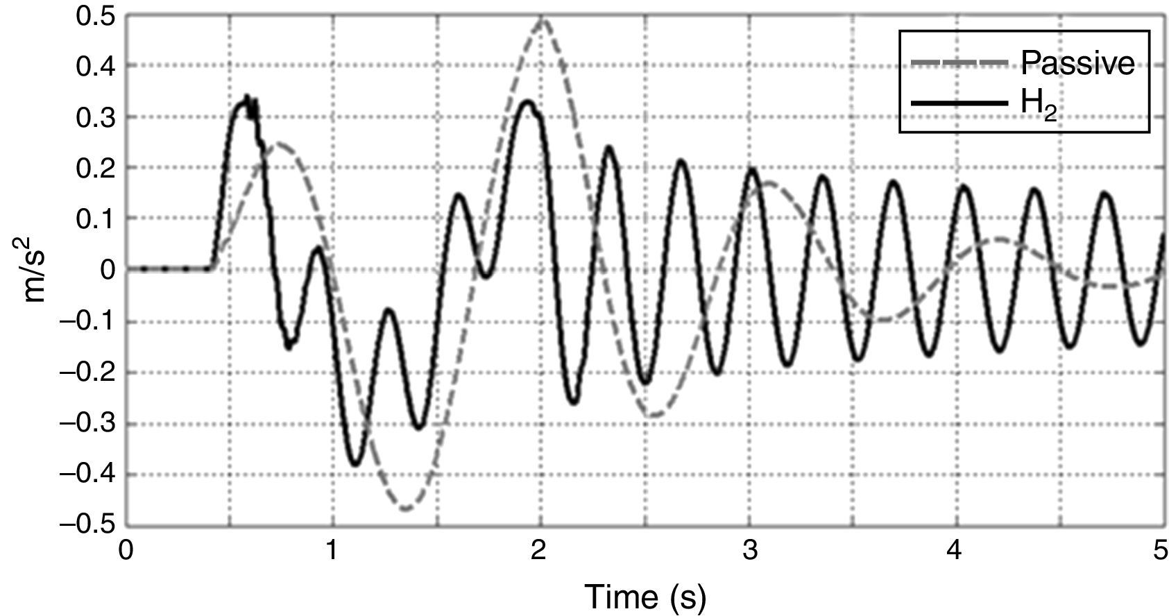
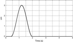
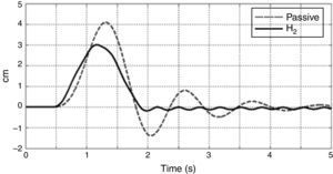
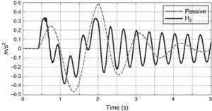
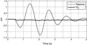
5.2

Tests in time domain

In addition to frequency domain tests, it is worthwhile to analyze suspension performance during transient response (time domain). This is usually tested by the automotive suspension's response when disturbance has the form of a road bump or a pothole. In general terms, the semi-active suspension should decrease the overshoot and settling time of sprung and unsprung masses’ displacement as well as for chassis acceleration. Present work includes the system's response for a road bump disturbance of 3.0 cm high, as illustrated in Figure 8.

Figure 8.

Disturbance in the form of a road bump profile.

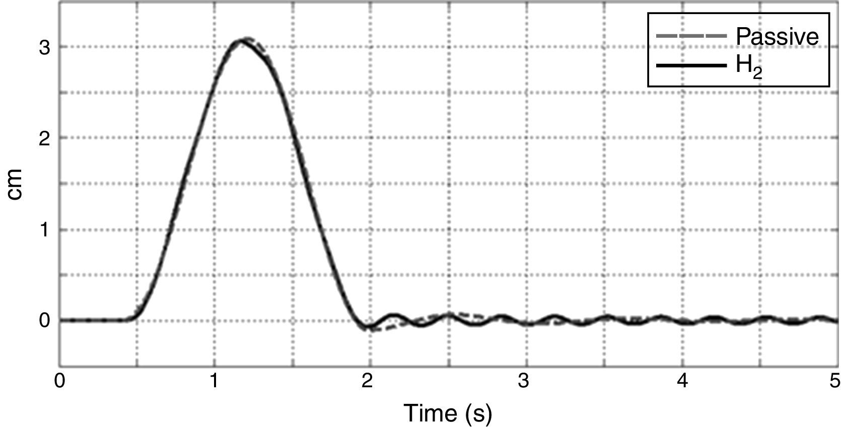
Even though disturbances do not have the same values, the idea is to carry out the tests in Tyan, Tu, and Jeng (2008), and Gao, Sun, and Shi (2010). Time domain results are presented in Figures 9–12.

Figure 9.

Chassis, or sprung mass displacement for the passive and H₂ controlled suspensions.

Figure 10.

Tire or unsprung mass displacement for the passive and H₂ controlled suspensions.

Figure 11.

Chassis acceleration for the passive and H₂ controlled suspensions.

Figure 12.

Suspension deflection for the passive and H₂ controlled suspensions.

Concerning chassis displacement in Figure 9, and suspension deflection in Figure 12, the semi-active solution considerably improves the passive suspension. In addition, tire displacement performance in Figure 10, is almost the same for both suspensions. In Figure 11, chassis acceleration is negatively affected because it presents oscillations that increase the steady state value of zero, but a positive aspect observed in the semi-active solution is that acceleration maximum peak values are slightly decreased. This is an opportunity area of this research effort.

6

Comparison with reported results

Even though, there is a lot of reported work regarding one-quarter vehicle suspensions, most of them restrict their results to time response. Not many articles refer to frequency domain tests or include one or two performance indexes. In Du (2009), a robust H_∞ controller is calculated for a semi-active suspension with an electro-rheological damper (Stanway, 1996). It obtains an outstanding result by improving the (x_s/x_p) relation in almost 83% with respect to a passive suspension. However, it does not include more performance criteria and no stability analysis can be completed.

The present work employs the frequency domain criteria reported in Sammier et al. (2003). More recent work, Poussot-Vassal et al. (2008) and Do et al. (2010), followed the same criteria with small adjustments. The former evaluates the indexes via their power spectral density (PSD) measure in the frequency domain, whereas the latter, reduces the relations (x_s/x_p) and (x_t/x_p) to be less than 1.8, and presents descriptive functions as well as PSD graphs. The performance criteria in, Poussot-Vassal et al. (2008) are the most similar to the reported ones here. More recently, Félix-Herrán et al. (2012) reported an H_∞ controller for a semi-active suspension. The obtained results were outstanding compared against the previous work included in this paragraph.

Even though, one-quarter vehicle parameters in the four previous articles are different, and not all the indexes are measured in the same manner, e.g., in this work, chassis acceleration considers the acceleration's rms value; an idea of the percentage of improvement with respect to passive suspension can be depicted in Table 3. The quantities are estimated according to obtained results in each case, and they are the percentage of improvement with respect to the passive suspension reported in each work. Note that reported percentages refer to the maximum value in each category, e.g., in Table 2, the maximum (x_s/x_p) for the passive suspension is 3.23, whereas the highest one for the H₂ approach is 1.91. The latter decreases the gain peak in 1.32 with respect to the former. This means an improvement of 40.8%.

Table 3.

Frequency domain results. Comparison among reported work and herein proposed suspension solution.

% of improvement with respect to passive case	H∞ (2003)^a	LPV/H∞ (2008)^b	LPV/H∞ (2010)^c	H∞ (2012)^d	H2 proposed herein
(xs/xp)	38.2	Not reported	12.1	46	40.8
(xt/xp)	Minor (≤5)	8	7	39.7	40
(xs–xt)	Not reported	16.2	8	65	61
Chassis acceleration	Minor (≤5)	18	25.4	Negative	Negative

a

Sammier et al. (2003).

b

Poussot-Vassal et al. (2008).

c

Do et al. (2010).

d

Félix-Herrán et al. (2012).

In Table 3, the herein outcome improves three out of four performance indexes. It behaves better regarding (x_s/x_p), (x_t/x_p) and suspension deflection. Chassis acceleration criterion is not enhanced with respect to the passive one, as well as the reported work in Sammier et al. (2003), Poussot-Vassal et al. (2008) and Do et al. (2010). However, the chassis acceleration result complies with the performance criterion as illustrated in Figure 6. This condition is the cost of a suspension system that meets the four frequency domain requirements.

The outcomes reported in this research improve three performance criteria. Along with the solution proposed in Félix-Herrán et al. (2012), the semi-active suspension approach in this research has outstanding results. Both solutions comply with comfort at high frequencies requirement, although neither of them improves the passive suspension performance in this category.

7

Conclusions and further work

Outcomes presented in Félix-Herrán et al. (2010) were extended with more advance control techniques that improved one-quarter vehicle suspension reported work. Under the testing conditions herein, obtained semi-active suspension system with an H₂ controller satisfies all stated frequency domain performance criteria. Moreover, the results obtained with an average city vehicle passive are considerably improved through a semi-active suspension. This approach is justified and proved to be a real solution that meets all stated requirements. Moreover, a comparison with reported work, Sammier et al. (2003), Poussot-Vassal et al. (2008) and Do et al. (2010) that follows the same performance criteria has been carried out. Solution proposed herein, performs adequately when is compared with reported work.

Insertion of MR damper dynamics enhances the presented results by a more exact behavior of the suspension system. Controller's output is a current value to the damper instead of a theoretical ideal force generated in an instant time.

Concerning rms chassis acceleration, compliance with the 8 h comfort boundary line in Wong (2001), is a requirement not included in previous work. However, if the lower MR damper input range is extended to 0.1 A, the damper will generate a smaller force, hence the rms acceleration value in Figure 6 could be decreased. This change will require an impact analysis on the other indexes, because the relation (x_s/x_p) and (x_s–x_t) will negatively be affected.

The herein case of study considers a completely measurable state vector. However, there could be unmeasurable variables. Future work is intended to work with a state observer, e.g., an estimator for displacements or velocities from sensors that measure acceleration.

Authors identify one limitation in this research that will be addressed in future work. Full scale vehicle's suspension model, i.e. a commercial vehicle is being developed as part of a more complete research effort where counter-phase and damper's passivity will be tested in real conditions. For now this research does not considers controller's saturation when disturbances have a magnitude outside prescribed range.

Actual work is been performed on half vehicle. The idea is to extend the present research to a more complex suspension model by adding the pitch dynamics.

Conflict of interest

The authors have no conflicts of interest to declare.

Acknowledgements

Authors are grateful to the Consejo Nacional de Ciencia y Tecnología (CONACYT) through the Sistema Nacional de Investigadores (SNI), in México; as well as Tecnológico de Monterrey through the Robotics focus group for supporting and funding this research.