Using the Monte Carlo Simulation Methods in Gauge Repeatability and Reproducibility of Measurement System Analysis

Abstract

Measurements are required to maintain the consistent quality of all finished and semi-finished products in a production line. Many firms in the automobile and general precision industries apply the TS 16949:2009 Technical Specifications and Measurement System Analysis (MSA) manual to establish measurement systems. This work is undertaken to evaluate gauge repeatability and reproducibility (GR&R) to verify the measuring ability and quality of the measurement frame, as well as to continuously improve and maintain the verification process. Nevertheless, the implementation of GR&R requires considerable time and manpower, and is likely to affect production adversely. In addition, the evaluation value for GR&R is always different owing to the sum of man-made and machine-made variations. Using a Monte Carlo simulation and the prediction of the repeatability and reproducibility of the measurement system analysis, this study aims to determine the distribution of %GR&R and the related number of distinct categories (ndc). This study uses two case studies of an automobile parts manufacturer and the combination of a Monte Carlo simulation, statistical bases, and the prediction of the repeatability and reproducibility of the measurement system analysis to determine the probability density function, the distribution of %GR&R, and the related number of distinct categories (ndc). The method used in this study could evaluate effectively the possible range of the GR&R of the measurement capability, in order to establish a prediction model for the evaluation of the measurement capacity of a measurement system.

1

Introduction

A number of different measurement methods have been developed to assess the precision and quality of products, and these mainly focus on the total variation of measurement, generally called measurement uncertainty [1]. In many manufacturing processes, parts are measured to ensure certain specifications are met. However, these measurements might be misleading if the measurement system itself is not adequate [2]. Measurement errors can be caused by the measurement instruments, appraisers, objects measured, or the measuring environment. In this context, gauge variability plays a key role in quality improvement because only with a gauge that has acceptable repeatability and reproducibility can the adequacy of a product's measurement process be determined. Therefore, a sound measurement system is an essential part of the total quality assurance programs used by many companies [3]. Evaluating a measurement system is an important aspect of many quality and process improvement activities [1], and in recent years, following the introduction of QS 9000/TS 16949 and the Six Sigma program, quality control personnel have begun to focus more heavily on the measurement systems they use, as well as on the problems of repeatability and reproducibility [4]. Repeatability is defined as the “variation in measurements obtained with one gauge being used for several times by one appraiser while measuring a characteristic on one part”. Reproducibility is defined as the “variation in the average of the measurements made by different appraisers using the same gauge when measuring a characteristic on one part” [5].

Montgomery and Runger [6] indicated that a measurement system should play an active role in the actions for quality improvement carried out by organizations, and that GR&R analysis should be used to identify the sources of variations within measurement processes and to quantify these variations. In order to reduce uncertainties, ISO/IEC 17025 [7] was formulated to evaluate Type I errors (α), which are the risk of manufacturers judging qualified products as defective ones, and Type II errors (β), which are the risk of consumers judging defective goods as qualified ones. In practice, a measurement system does not always obtain the exact dimensions of the part, but gives measurements that deviate to some extent from the true value [1]. In addition, there is also some uncertainty about inaccuracies in the measurements, because accurate measurements of these errors are also difficulty to obtain [3]. Type II errors require particular attention, because they could affect directly subsequent manufacturing processes and cause customer complaints or increase quality failure costs. AIAG [8] indicated that Statistical Process Control (SPC) is normally used to monitor the measurement capability of a process, and that SPC is not merely a useful tool, but an essential part for quality assurance, because without good evaluation of measurement capability and reliability, the measured data cannot be considered unreliable [9].

Previous research on this topic has examined mainly how firms undertook analyses of their measurement systems [3,4,10] or presented comparisons of various measurement evaluation methods. For instance, statistical methods have been used to predict how to apply an evaluation method or whether there were any interactions between researchers and products [1,2,11]. Using the medium, ‘Average and Range’ analysis in the MSA Reference Manual [12] to evaluate the statistical requirements of GR&R, the current study applies a Monte Carlo simulation to predict the repeatability and reproducibility of the measurement system analysis. It does this by judging the distribution of %GR&R and ndc, determining the possible distribution area and evaluating its probability with statistical data, as well as predicting the measurement uncertainty. The results of this analysis could serve as the foundation for the evaluation and continuous improvement of a company's measurement systems, enabling more effective monitoring of products and the achievement of better quality specifications and thus, greater customer satisfaction.

2

Literature review

2.1

Measurement system analysis

Measurement system analysis (MSA) is a systematic procedure that identifies the components of variations in the precision and accuracy assessments of the measuring instruments used in a measurement system [13]. The aims of MSA are to: (1) determine the extent of the observed variability caused by a test instrument, (2) identify the sources of variability in a testing system, and (3) assess the capability of a test instrument [14].

MSA is an important element both of Six Sigma and of the ISO/TS 16949 standards [15]. It is used to evaluate the reliability of some important input and major output data in the manufacturing process, understanding the variations caused by people, machines, materials, methods, or the environment, and then using the analyzed data as a reference for improvements [1].

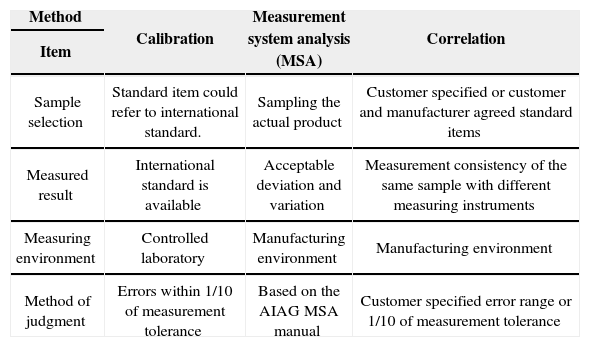
Since the adoption of MSA by three major Northern American automobile manufacturers in 1991, the entire industry has also begun to use this approach. In addition, with the various problems that could arise during the manufacturing of high-technology, function-oriented, and ultra-precision products, the precision of measuring instruments has received increased attention in the literature [2]. If the measurement results are not accurate, then it is more likely that poor quality products will be supplied to customers. For this reason, manufacturing and examination processes both require a precise measurement system in order to maintain product quality and to enhance a firm's reputation. General evaluations of measurement systems include calibration, MSA, and correlation, and a summary of these methods is presented in Table 1.

Table 1.

Evaluation methods of measurement systems.

Method	Calibration	Measurement system analysis (MSA)	Correlation
Item
Sample selection	Standard item could refer to international standard.	Sampling the actual product	Customer specified or customer and manufacturer agreed standard items
Measured result	International standard is available	Acceptable deviation and variation	Measurement consistency of the same sample with different measuring instruments
Measuring environment	Controlled laboratory	Manufacturing environment	Manufacturing environment
Method of judgment	Errors within 1/10 of measurement tolerance	Based on the AIAG MSA manual	Customer specified error range or 1/10 of measurement tolerance

Source: Barrentine [16]

MSA applies statistics and charts to implement a simple experimental design and statistical analyses of measurement system errors, and assesses variations in the measuring instruments and the work of on-site inspectors [10]. If the errors that occur with the measuring instruments and the inspectors are significant, then the reliability of the data recorded in the measurement process will be in doubt. The ideal measurement system should have statistically zero mistakes with regard to the measured product [1], although this is not possible in practice.

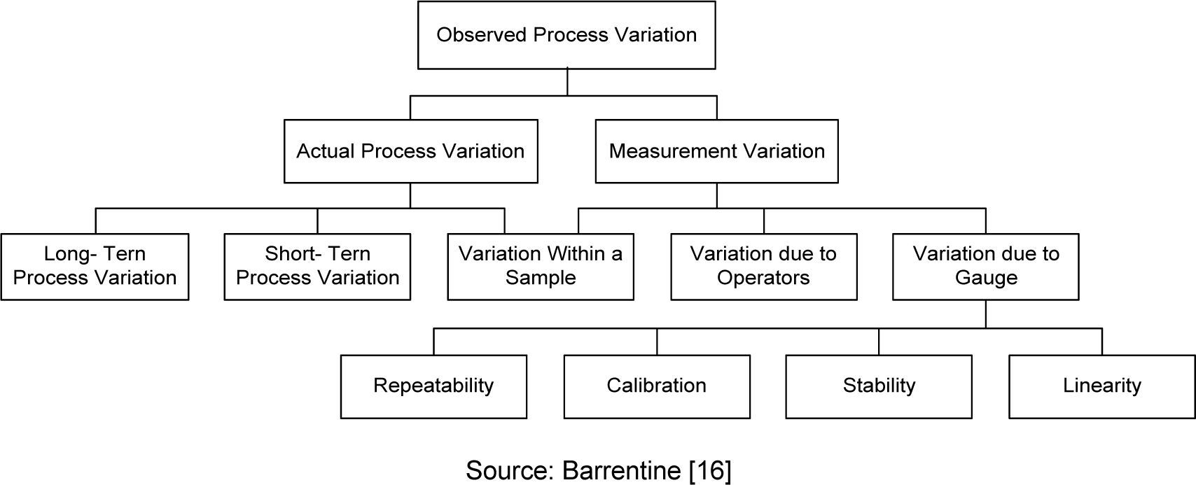
Three basic statistics arise from measurement. First, the measurement system should have an appropriate degree of discrimination with the best discrimination showing 1/10 of the total process 6α, not 1/10 of the traditional tolerance. Second, the measurement system should have statistical evaluation stability at a specific time, and this applies not only to the stability of the measuring instruments, but also to reproducibility. Third, the statistical generalization of the measurement error, or the variation, should achieve consistency within the expected range, which could then be used in the process analyses or control. The measurement system error for variable instruments is classified with regard to accuracy and precision. Here, accuracy refers to the difference between the measured value and the real value of the sample, whereas precision is the measurement variation resulting from the same equipment repeatedly measuring the same sample. In any measurement system, one or two errors are likely to appear. Furthermore, precision is divided into two elements: repeatability and reproducibility. The former is the variation caused by a measurement instrument, whereas the latter is the variation resulting from a measurement system. The MSA manual [12] proposes three variable gauges to confirm repeatability and reproducibility: the Range, the Average and Range, and ANOVA (Analysis of Variance) methods. Barrentine [16] presented a complete introduction of the Average and Range method to observe the composition of the process variations, as summarized in Figure 1.

Figure 1.

Analyses of process variation.

Source: Barrentine [16]

2.2

GR&R studies

Measurement errors could be caused by the measurement instruments, measuring personnel, measured objects, and the measuring environment. Measurement data become inaccurate without a precise measurement system for assessment, evaluation, and monitoring, leading to inaccurate calculations of process capabilities [9]. GR&R studies are performed according to the QS 9000 standards. as stated in MSA [17], in order to assess the suitability of a gauge. Both QS 9000 and ISO/TS16949 in MSA define GR&R as acceptable criteria.

Pan [4] indicated that there were three evaluation methods commonly used to study GR&R in industry and academia. First, Mandel [18] used the expected mean squares to find the total variation of measurement based on the concept of ANOVA. Second, Montgomery and Runger [19] proposed Classical GR&R. This uses the mean and range to estimate the total variation of measurement of GR&R, which obtains an estimate of the standard deviation for GR&R. Third, three major American automobile companies, GM, Ford, and Chrysler, developed the Long Form approach introduced in the MSA manual [12]. This method is used to estimate the total measurement variation of GR&R and the precision value to tolerance (P/T) ratio, and it was designed especially for use by quality practitioners without a statistical background.

Feng et al. [11], Mandel [18], and McNeese and Klain [20] also mentioned the concepts of repeatability and reproducibility. Repeatability is defined as repeatedly measuring the same product in the same laboratory and measuring the variation in the results, whereas reproducibility is defined as repeatedly measuring the same product in different laboratories and measuring the variation in the results. Tsai [21] defined repeatability variation as the same appraiser repeatedly measuring the same sample in the same environment and obtaining the measurement variation, which is the variation produced by the gauge in the process of measuring. He further defined reproducibility variation as different appraisers measuring the same sample in the same environment and acquiring the measurement variation. Comparing Mandel [18] and Tsai [21], the reproducibility variation in the former was caused by different appraisers, whereas it was caused by different laboratories in the latter. McNeese and Klain [20] stated that the variation analyses and sampling techniques in measurement systems are the elements that could be used to improve measurement capability, and that product and measurement variation are the two factors that make up the overall variation. In this case, changes in variation should be emphasized in the measuring process. They also stated that a capable measurement system, as defined by Ford, should emphasize the statistical control of the mean value and variance.

Here, the observed mean value in the process should approach the true value of the product, while the measurement variation should be less than 10% of the total process variation. The capability of precision (CP) is shown in formula (1), in which tolerance is the specification limit and the standard deviation (σ) is the process standard deviation of the observed value.

The three major US automobile companies, Chrysler, Ford, and GM, published the MSA Reference Manual in 1991, which set out the Average and Range method, which has since become widely accepted by academia and industry. However, there are a number of problems with this approach, such as a lack of charts in the evaluation formula for part variation, and no measurement capacity indicators. Therefore, James and Finderne [22] proposed a mean graph, range graph, and scatter plot to improve the Average and Range method. Barrantine [16] presented a complete introduction of the Average and Range method in the MSA manual, where four or more appraisers could be used, and GR&R analysis of a measurement system could be carried out with less than ten sample parts or only one appraiser. He also proposed an acceptable value to judge a gauge system when measuring precision, namely %GR&R, as shown in formula (2). In this system, value < 10% is defined as an excellent system for the gauge, values of between 10% and 20% are deemed as an appropriate measurement, values of between 20% and 30% are at the edge of acceptance, and values > 30% are seen as unacceptable, and thus, requiring readjustment.

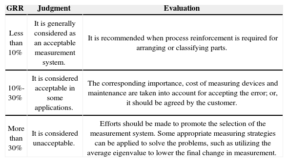
Montgomery and Runger [19] stated that ANOVA is more accurate than the Average and Range method because it takes the interaction between the operator and the sample part into account. However, although either the Average and Range method or ANOVA can be utilized when choosing MSA GR&R, the standard values for accuracy need to be the same. The acceptable general proportions for Precision Width Error mentioned in the MSA manual [12] are shown in Table 2. These suggest that the number of distinct categories (ndc) could distinguish the largest number of categories when choosing the measurement system to process the data, and that this should be greater than five for the analyzed data to be considered reliable. The calculation formula for ndc is described in the following research methods.

Table 2.

Acceptable general proportions for precision width error.

GRR	Judgment	Evaluation
Less than 10%	It is generally considered as an acceptable measurement system.	It is recommended when process reinforcement is required for arranging or classifying parts.
10%-30%	It is considered acceptable in some applications.	The corresponding importance, cost of measuring devices and maintenance are taken into account for accepting the error; or, it should be agreed by the customer.
More than 30%	It is considered unacceptable.	Efforts should be made to promote the selection of the measurement system. Some appropriate measuring strategies can be applied to solve the problems, such as utilizing the average eigenvalue to lower the final change in measurement.

Source: AIAG MSA Manual [11]

2.3

Monte Carlo simulation

The Monte Carlo simulation, which originated from statistical sampling, was first presented by Metropolis and Ulam [23]. It has been widely used to model complex systems [24] with several authors adopting it to measure system reliability owing to its advantages of convenience and accuracy [25]. A Monte Carlo simulation requires the following elements [26]: (1) a probability density function (p.d.f.); (2) a random number generator to provide random numbers; (3) a sampling prescription, sampled from a specified p.d.f. with an available unit interval random number; (4) calculation, in which the output results need to be given as a total value; (5) miscalculation, in which the relationship between the number of times statistical errors occur and the functions of other numbers needs to be confirmed; (6) a variation reducing technique, to reduce the time needed to calculate the Monte Carlo simulation; and (7) horizontal and vertical integration, to apply the Monte Carlo simulation effectively to an advanced computing system structure.

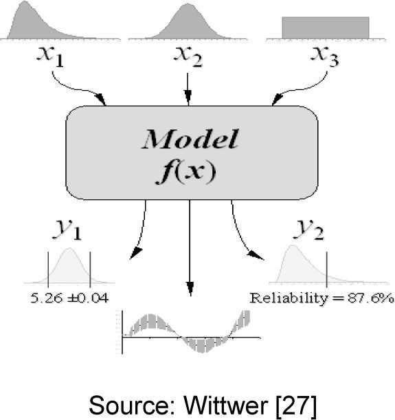
The Monte Carlo simulation is a method for evaluating iteratively a deterministic model using sets of random numbers as inputs. This method is often used when the model is complex, nonlinear, or involves more than just a couple of uncertain parameters [26]. The Monte Carlo simulation is categorized as a sampling method because the inputs are generated randomly from probability distributions to simulate the process of sampling from an actual population. Therefore, we try to choose a distribution for the inputs that matches most closely the data we already have, or best represents our current state of knowledge. The data generated from the simulation can be represented as probability distributions (or histograms) or converted to error bars, reliability predictions, tolerance zones, and confidence intervals (See Figure 2) [27].

Figure 2.

Output reliability, tolerance, and confidence interval in a Monte Carlo simulation.

Source: Wittwer [27]

The basic principle of a Monte Carlo simulation lies in defining p.d.f. with the probability of all possible results. The p.d.f. then becomes the cumulative probability function, the value of which is adjusted to the maximum level of 1, called normalization. This also shows that the total probability of all events is 1, which means that the simulation could be used for both random sampling and real problems. Using the simulation with the p.d.f. input, the reliability, tolerance, and confidence interval of real problems can be simulated. Five basic steps are needed to carry out a Monte Carlo simulation, as follows [28]:

• Step 1:

  Generate a model with parameter y = f(x₁, x₂, …, x_q)

• Step 2:

  Generate a set of random number inputs xi1, xi2, …, xiq

• Step 3:

  Evaluate the model with the saved result yi

• Step 4:

  Repeat Steps 2 and 3, i = 1 to n

• Step 5:

  Analyze the statistical results and confidence intervals

Random numbers are required at the beginning of a Monte Carlo simulation, and while these used to be generated by physical methods, such as dice, playing cards, and roulette wheels, these had the drawbacks of being slow and non-reproducible. The Rand Corporation developed a random number table in 1955, which was composed of millions of numbers. Although these random numbers could be reproduced, the process was slow, and when more simulation events were required, this method was insufficient. In contrast, the Mid-Square Method calculates the square of a four-figure number, or even a six- or two-figure number, although the numbers generated from this method can only be called pseudo-random or quasi-random, because they are fixed numbers generated from a certain function (without randomness). Chaitin [29] indicated that random numbers should satisfy the requirements of being: (1) uniformly distributed, (2) statistically independent, and (3) reproducible. The Linear Congruential Method (LCG), first proposed in Lehmer [30], is presently the most commonly utilized method to achieve this. The basic principle of LCG can be seen in formula (3). The initial x of the random number generator requires a “seed value”. Using formula (3) for the calculation, it then becomes the new ISEED with the random number, and uniform random numbers between (0,1) can be acquired by continuing this process. In this study, Crystal Ball (CB) software is used for to undertake the Monte Carlo simulation, as shown in formula (4). There is no “seed value” used for the multiplicator at the beginning of this process because the LCG generator utilizes an iteration equation, and because the length period of the generator is 2,147,483,646, showing that the number could be reproduced after several billions of tests. Law and Kelton [31] presented a detailed explanation of this method.

Most software applies a combination of two or more random number generators to produce a new random number generator [32]. Using the LCG method (or another method) to generate numbers between 0 and m-1, the numbers are then divided by m to become random numbers between 0 and 1. This is similar to the random variable of U(0,1), and the other distributed random numbers generated by U(0,1) are uniform to ensure that the random numbers have the characteristic of U(0,1). The results are then tested using the goodness of fit, including the Chi-square goodness of fit and Kolmogorov-Smirnov tests. The Chi-square test is mainly used for dealing with the test of the categories, and this study applied the Chi-square goodness of fit to ensure the %GR&R probability distribution, as shown in formula (5).

o_i: Observed frequency in each category

e_i: Expected frequency in the corresponding category

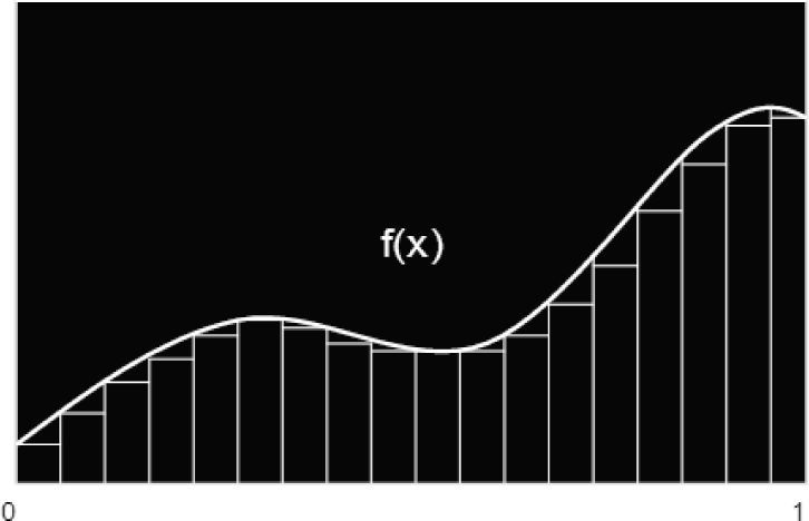
Furthermore, the Monte Carlo numerical integration can be used for the calculation of numerical integration, and the probability distribution area can be calculated using random numbers. When integrating a number, the [0,1] interval can be simply divided [33]. M parts can be evenly divided to compose the area with the total being 1, i.e., 100%, as in formulae (6) and (7). In other words, Xn can be divided evenly into n = 1, 2, …, M parts with a random generator. When M is large enough, Xn is the set with evenly divided parts in [0,1], as in formulae (8) and (9), and the Xn wave-constructed area is as shown in Figure 3. As a result, it is considered complete and accurate to apply a Monte Carlo simulation to predict or evaluate random numbers.

Figure 3.

f(x) area divided by M equal parts.

3

Research method

Based on the Average and Range analysis in the MSA manual [12], 90 data with ten sample parts, three appraisers, and three measuring events were computed using a Monte Carlo simulation. Pen [3, 4] noted that the Average and Range analysis is widely applied in industry, and thus, this study uses the same approach to evaluate GR&R, in order to verify the measurement capability and quality of the measuring instrument, as well as to evaluate the acceptability of the measurement system.

The research procedure is as follows:

• 1.

  Select ten sample parts, numbered 1 to 10, which must completely represent the range of the process variation.

• 2.

  Select three appraisers, known as A, B, and C.

• 3.

  The appraisers randomly and repeatedly measure the sample parts three times. The measurement results cannot be seen by the personnel. Thirty sets of data are generated from each appraiser, generating 90 data sets in total.

• 4.

  Having completed the measurement, the three values from measuring each sample are calculated to produce the average and the range, such that ten averages and ten ranges are generated by each appraiser.

• 5.

  The values from each appraiser measuring each sample part are the sample averages, and ten of these are averaged as Rp.

• 6.

  Each appraiser generates ten averages, for which the average is obtained as AverageX_A, AverageX_B, and AverageX_C. The average of ten ranges generated by each appraiser is acquired as R¯a, R¯b and R¯c.

• 7.

  Calculate R¯¯ and X¯DIFF, as in formulae (10) and (11).

  
  

• 8.

  Repeatability is the equipment variation (EV), which is determined by multiplying the average range (R¯¯) by a constant (K₁). K₁ depends upon the number of trials used in the gauge study, and is equal to the inverse of d2*, which is obtained from the MSA manual [12] Appendix C, page 187. d2* is dependent on the trial number (m) and the part number multiplied by the appraiser number (g). Therefore, EV is calculated using formula (12). In this research, the measurement is carried out three times. According to the MSA manual, K₁ is equal to 0.5908, and reproducibility is the appraiser variation (AV), which is determined by multiplying the maximum average appraiser difference ((X¯DIFF)) by a constant (K₂). K₂ depends upon the number of appraisers used in the gauge study, and is the inverse of d₂ which is obtained from the MSA manual [12] Appendix C, page 187. d2* is dependent on the appraiser number (m) and g = 1 because there is only one range calculation. As the appraiser variation is contaminated by the equipment variation, it must be adjusted by subtracting a fraction of this variation, and thus, AV is calculated by formula (13). There are three appraisers in this research, and based on the MSA manual, K₂ is equal to 0.5231, sample “n” is 10, and measurement “r” is 3.

  
  

• 9.

  The GR&R of the measurement system calculated by repeatability and reproducibility is shown as formula (14).

  

• 10.

  Calculate the process variation (PV) by multiplying the average of the sample parts by a constant (K₃). K₃ is determined by the number of the sample parts in the measurement, and is the inverse of d₂^*, which can be obtained from the MSA manual. d2* is determined by the number of appraisers and the number of subsets, as in formula (15). There are ten sample parts in this study, such that K₃ = 0.3146, and from the MSA manual:

  

• 11.

  Add the square of GR&R and the square of PV. The total variation (TV) is the square root of the sum, as in formula (16).

  

• 12.

  %GR&R is the percentage of GR&R in the total variation, as in formula (17).

  

• 13.

  Finally, confirm the reliable ndc of the measurement system. Wheeler and Lyday [34] indicated that ndc is the number covering the 97% reliable interval that is not overlapped by expected product variation, as in formula (18). ndc must be rounded as an integer.

  

With regard to the measurement uncertainty mentioned in the MSA manual, it is the degree of scatter of the measured results, and is normally shown by the standard deviation after several repeated measurements. Using statistical methods, some of the results can be estimated from the standard deviation calculated using the real data, whereas others are estimated from the standard deviation calculated using the assumed probability distribution based on experience or other information.

The basic formula is shown as (19), where U is the expanded uncertainty between the measured object and the measured result. Expanded uncertainty is the distribution coefficient (K) with a normal distribution, such that the standard deviation of the combined standard error (Uc) or combined error is multiplied by an expected reliability range in the measuring process. ISO/IEC Guide 98–3 [35] states that the distribution coefficient (K = 2) represents 95% uncertainty of the normal distribution. Formula (20) shows that the measured value is located in the interval ±2σ away from the average, i.e., the 95% reliability interval. The collaborative assessment experiment in ISO 5725–1:1994 [36] further notes that the probability standard approaches 95% when many experiments are used in a precision test. Consequently, assuming the defined range for the measured value is ±2σ, the basic statistical model used to estimate the precision of the measurement is shown as formula (21). This shows that with the sum of the total average and repeatability, and the sum of the deviated values in the laboratory and repeatability, the random errors generated from each measurement can rationally result in numerical dispersion, and that the random error can be combined with the Monte Carlo simulation to determine the probability.

for

m: general mean

B: laboratory component of the bias under repeatability conditions

e: random error under repeatability conditions

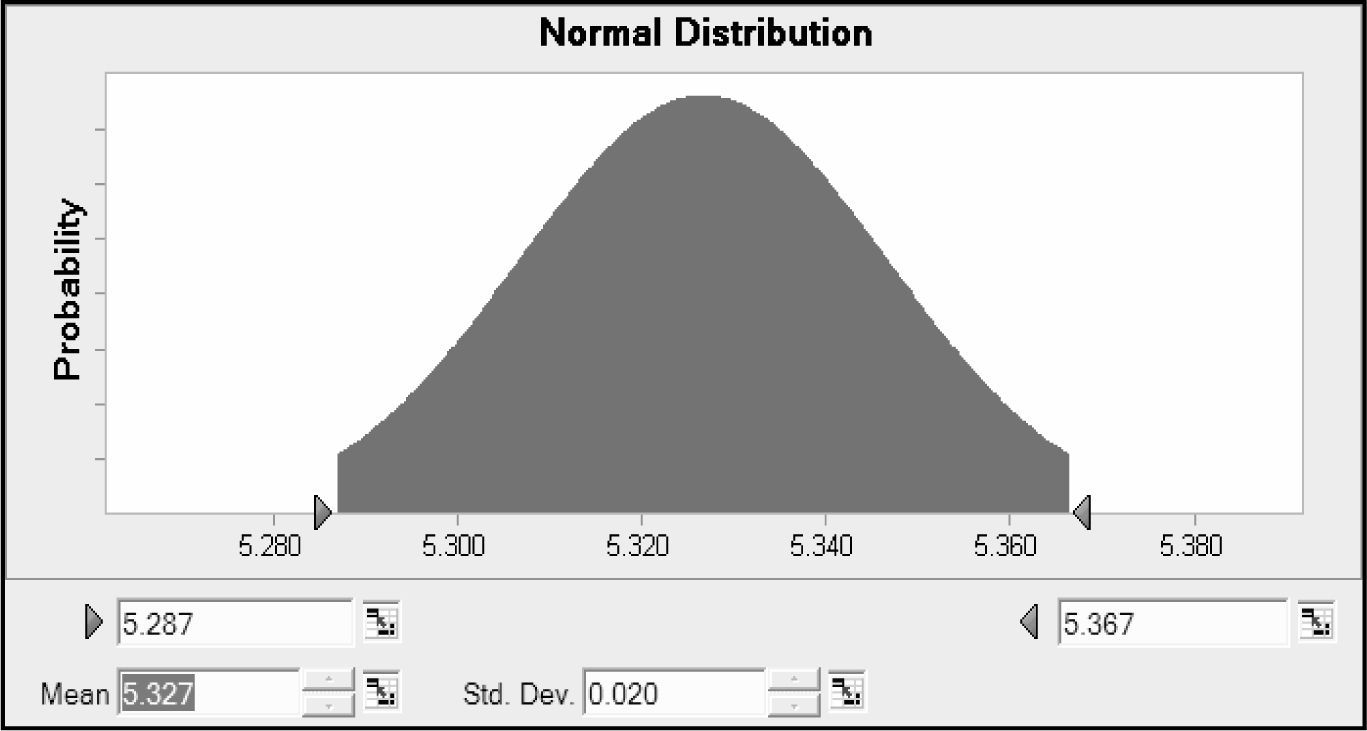
Combining the Average and Range analysis in MSA with a Monte Carlo simulation, ten sample parts were selected and each sample part was measured three times by three appraisers to obtain nine measurements. There was no variation for the single parts, but different variation values appeared for each measurement. Based on measurement uncertainty, rational numerical dispersion could result from the measurement. In this case, the average and the standard deviation of the nine measurements of each part were calculated. Based on the results of measurement uncertainty, the measurement was normally distributed in the 95% reliable interval (±2σ). In addition, the nine measurements also defined the distribution probability of the Monte Carlo simulation as being ±2σ away from the normal distribution interval. The relevant normal distribution can be seen in Table 3. Substituting the p.d.f. of the normal distribution, as in formula (22), the results are shown in formula (23) and Figure 4. When calculating AV, the setting restriction, as in the MSA manual, is that AV is 0 when the square root value is negative. With the Crystal Ball software, a total of 90 measurements with ten sets and nine data for each set were used to generate random numbers with a Monte Carlo simulation. Furthermore, with the 10,000 tests defined in probability theory applied to formulae (17) and (18), the cumulative probability distributions of %GR&R and ndc were obtained. The analysis and the evaluation obtained from this process are used as a reference later in this study.

Table 3.

Calculating the Monte Carlo simulation settings of the nine measurements.

Operator	A			B			C			Monte Carlo Simulation Spec.
Measurement	1^st	2^nd	3^rd	1^st	2^nd	3^rd	1^st	2^nd	3^rd	Mean (μ)	SD(σ)	x
Part Sample												Max (μ+2σ)	Min (μ−2σ)
Sample No.1	5.32	5.32	5.32	5.34	5.34	5.36	5.30	5.34	5.30	5.327	0.020	5.367	5.287

Remark: Based on resolution being 1/10 of tolerance, the setting is calculated to the next figure of the original measurement.

Figure 4.

Sample No.1 probability distribution of the measurements.

Having combined the expressions established in this study using Crystal Ball, a Monte Carlo simulation was implemented 10,000 times for the 10,000 data of %GR&R and ndc, which was similar to executing the measurement system analysis 10,000 times. By evaluating the original area of the measurement system and the judgment suggested by the MSA manual, the probability distribution and the possible probability of %GR&R were derived. The most appropriate normal probability distribution was then calculated using the Chi-square goodness of fit test.

4

Case verification and analysis

To verify the method we proposed, we used two case studies of an automobile parts manufacturer and selected as the subject for three appraisers, ten sample parts, and three-time measurements. In case study 1, ten indicator switches were selected as the samples, and the thickness of a part of the indicator switch was measured. In case study 2, ten precision bearings were selected, and the width of a part of the precision bearing was measured. The detail is described below.

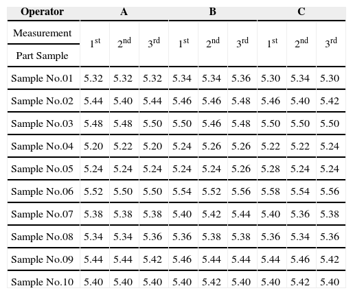
4.1

Case study 1

The first case studied was the dial indicator, coded MX-01, which had an obtained precision of 0.01 mm. Three appraisers, A, B, and C, were selected. Ten online-produced indicator switches were selected and the thickness of a part of the indicator switch was measured. Each appraiser measured the selected sample parts three times, as shown in Table 4.

Table 4.

Recorded measurements of case 1.

Operator	A			B			C
Measurement	1^st	2^nd	3^rd	1^st	2^nd	3^rd	1^st	2^nd	3^rd
Part Sample
Sample No.01	5.32	5.32	5.32	5.34	5.34	5.36	5.30	5.34	5.30
Sample No.02	5.44	5.40	5.44	5.46	5.46	5.48	5.46	5.40	5.42
Sample No.03	5.48	5.48	5.50	5.50	5.46	5.48	5.50	5.50	5.50
Sample No.04	5.20	5.22	5.20	5.24	5.26	5.26	5.22	5.22	5.24
Sample No.05	5.24	5.24	5.24	5.24	5.24	5.26	5.28	5.24	5.24
Sample No.06	5.52	5.50	5.50	5.54	5.52	5.56	5.58	5.54	5.56
Sample No.07	5.38	5.38	5.38	5.40	5.42	5.44	5.40	5.36	5.38
Sample No.08	5.34	5.34	5.36	5.36	5.38	5.38	5.36	5.34	5.36
Sample No.09	5.44	5.44	5.42	5.46	5.44	5.44	5.44	5.46	5.42
Sample No.10	5.40	5.40	5.40	5.40	5.42	5.40	5.40	5.42	5.40

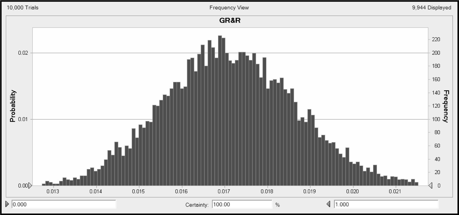
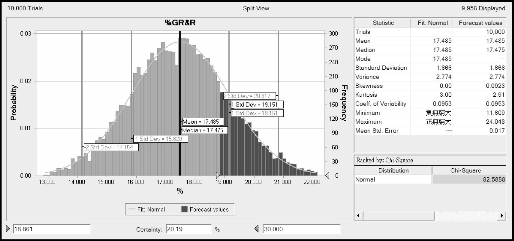
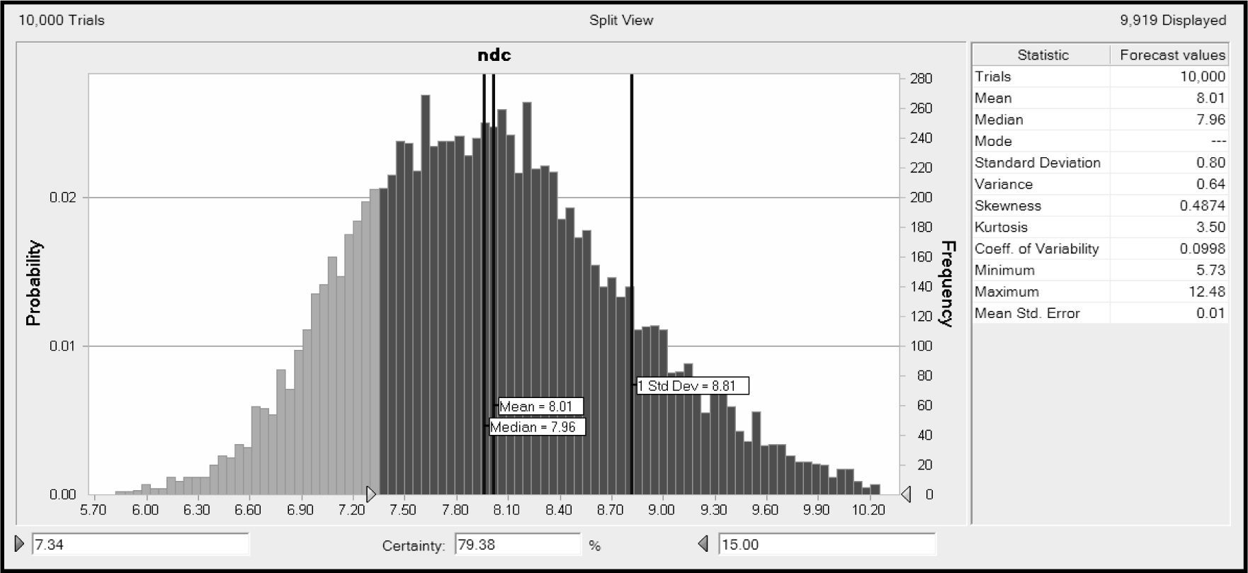
With the Average and Range analysis in the MSA Manual, a GR&R of 0.019 was obtained; the %GR&R, which was used to judge the measurement system, was 18.861% and the ndc was 7.342, which was rounded to 7. These values were then used to evaluate the measurement system analysis with a Monte Carlo simulation. GR&R was further input into the Crystal Ball software for 10,000 runs of the Monte Carlo simulation. The simulated distributions obtained thus for GR&R, %GR&R, and ndc, as well as the relevant data, are shown in Figures 5, 6, and 7.

Figure 5.

Simulated GR&R distribution of case 1.

Figure 6.

Simulated %GR&R distribution of case 1.

Figure 7.

Simulated ndc distribution of case 1.

Figure 5 shows the distribution of GR&R after 10,000 simulations. The original value of 0.019 is located on the right. As %GR&R is GR&R divided by the total variation, the %GR&R is therefore on the right. Further analyzing the %GR&R distribution in Fig. 6, the %GR&R is between 13% and 22% and thus, the automobile part was not a critical one. Based on the standard %GR&R specifications of 10% to 30%, shown in Table 2, it was found that MSA would always conform to the specifications. The results of the Chi-square test show that the %GR&R distribution was normal. The average of the 10,000 simulations was 17.485%, the standard deviation was 1.666%, and the original value was 18.861%, which was within +1α. As a result, the original value of 18.861% was judged to be in the +1α range. The probability of being larger than 18.861% was only 20.19%. As the %GR&R distribution was normal and the average of the test was 17.485%, the standard error of the mean (SEM) was further analyzed to produce the standard error of the output data, 0.017. The smaller the standard error, the greater the reliability and thus, the %GR&R was revised down to 17.485%.

The ndc distribution in Figure 7 was analyzed further. As an integer was required for the ndc, the distribution was not tested. Figure 7 shows the ndc distribution with 10,000 GR&R simulations. Based on the ndc specifications, an ndc of 5 is acceptable.

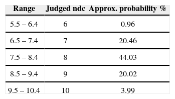
The original value of 7.342 is located on the left and the probability of being larger than 7.34 was 79.38%. Thus, the decision value can be revised up. As the real ndc was rounded to 7, the value was analyzed with integers in this study. Table 5 shows the ndc values with 10,000 simulations, rounded to one decimal point. Most values, about 44.03%, were located between 7.5 and 8.4, which were rounded to 8. The original value 7 accounted for only 20.46% of the results, only half of that of 8. Thus, the ndc was revised up to 8.

Table 5.

Proportion of ndc of case 1.

Range	Judged ndc	Approx. probability %
5.5 – 6.4	6	0.96
6.5 – 7.4	7	20.46
7.5 – 8.4	8	44.03
8.5 – 9.4	9	20.02
9.5 – 10.4	10	3.99

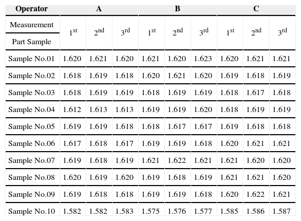
4.2

Case study 2

The second studied case was the dial indicator, coded MX-03 with a precision of 0.001 mm. Three appraisers, A, B, and C, were selected. Ten online-produced precision bearings were selected and the width of a part of the precision bearing was measured. Sample No. 10 was the same product but the width was measured on a different part of it and thus, there was a significant numerical difference from Sample No.01 to Sample No.09. Each appraiser measured the selected sample parts three times and the measurements are shown Table 6.

Table 6.

Recorded measurements of case 2.

Operator	A			B			C
Measurement	1^st	2^nd	3^rd	1^st	2^nd	3^rd	1^st	2^nd	3^rd
Part Sample
Sample No.01	1.620	1.621	1.620	1.621	1.620	1.623	1.620	1.621	1.621
Sample No.02	1.618	1.619	1.618	1.620	1.621	1.620	1.619	1.618	1.619
Sample No.03	1.618	1.619	1.619	1.618	1.619	1.619	1.618	1.617	1.618
Sample No.04	1.612	1.613	1.613	1.619	1.619	1.620	1.618	1.619	1.619
Sample No.05	1.619	1.619	1.618	1.618	1.617	1.617	1.619	1.618	1.618
Sample No.06	1.617	1.618	1.617	1.619	1.619	1.618	1.620	1.621	1.621
Sample No.07	1.619	1.618	1.619	1.621	1.622	1.621	1.621	1.620	1.620
Sample No.08	1.620	1.619	1.620	1.619	1.618	1.619	1.621	1.621	1.620
Sample No.09	1.619	1.618	1.618	1.619	1.619	1.618	1.620	1.622	1.621
Sample No.10	1.582	1.582	1.583	1.575	1.576	1.577	1.585	1.586	1.587

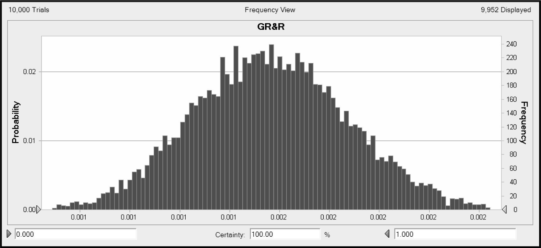
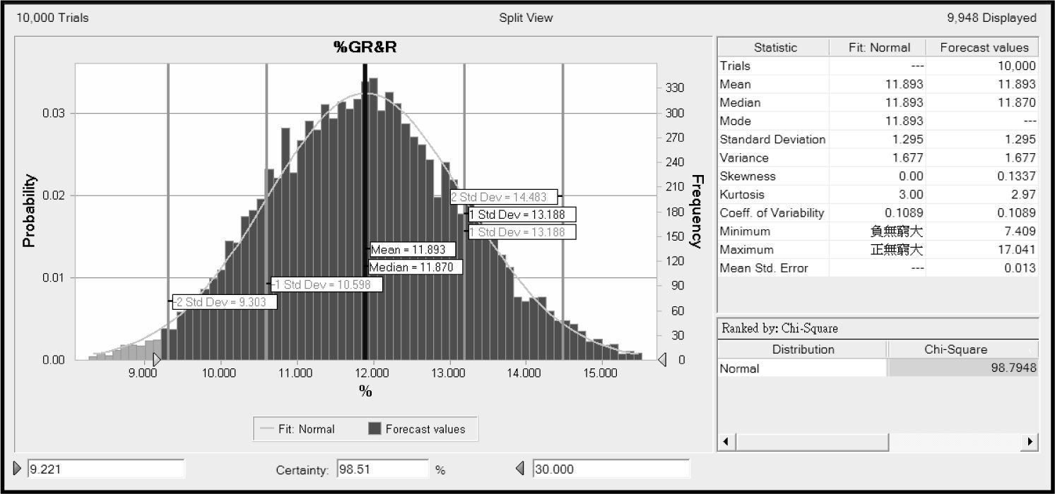
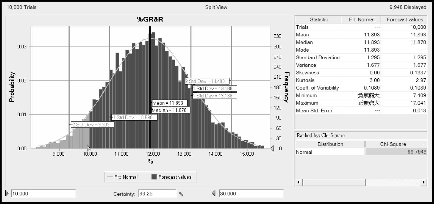
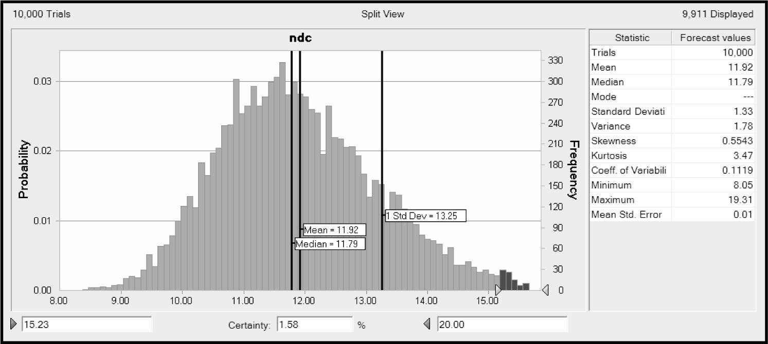
With the Average and Range analysis in the MSA Manual, the GR&R was found to be 0.001; the %GR&R, which was used to judge the measurement system, was 9.221%; and the ndc was 15.225, which was rounded to 15. These values were then used to evaluate the measurement system analysis with a Monte Carlo simulation. GR&R was further input into the Crystal Ball software for 10,000 Monte Carlo simulations. The simulated distributions obtained for GR&R, %GR&R, and ndc, as well as the relevant data, are shown in Figures 8, 9, 10, and 11.

Figure 8.

Simulated GR&R distribution of case 2.

Figure 9.

Simulated %GR&R distribution (1) of case 2.

Figure 10.

Simulated %GR&R distribution (2) of case 2.

Figure 11.

Simulated ndc distribution of case 2.

Figure 8 shows the distribution of GR&R after 10,000 simulations. The original value of 0.001 was located on the left. As %GR&R was GR&R divided by the total variation, the %GR&R was therefore judged on the left. Analyzing further the %GR&R distribution in Fig. 9, the %GR&R was predicted to be distributed between 8% and 16%. This automobile part is a precision critical part, and poor tolerance could cause turning problems when driving. Therefore, the %GR&R was regulated to less than 10%, and based on Table 2, the standard %GR&R specifications should also be less than 10%. However, the first problem was the judging limit of the %GR&R specification, 10%. The probability of the original %GR&R being higher than 9.221% was 98.51%, as shown in Figure 9.

Moreover, with the judging limit of 10%, the probability of it being higher than 10% was 93.25%, as seen in Fig. 10. Therefore, the %GR&R was revised up. With the Chi-square test, the %GR&R distribution was normal. The average of the 10,000 simulations was 11.839%, the standard deviation a 1.295%, and the original value 9.221% being out of −2α. As a result, the reliability of the original value 9.221% was rather low. Moreover, the %GR&R distribution was normal, the average of the distribution tests was 11.839%, and the standard error of the mean (SEM) was 0.013. The lower the standard error, the greater the reliability and thus, the %GR&R was revised up to 11.839%, especially as the automobile part was a precision critical one. The original standard of within a 10% limit was thus exceeded, and the capability of the measurement system was improved.

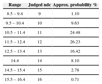
The ndc distribution in Figure 11 was analyzed further. As an integer was required for ndc, the distribution was not tested. Figure 11 shows the ndc distribution with 10,000 GR&R simulations. Based on the ndc specifications, an ndc of 5 is acceptable. The original value 15.225 was located on the right, and as the probability of it being larger than 15.225 was only 1.58%, the decision value should therefore be revised down. As the real ndc was rounded to 15, the value was analyzed using integers. Table 7 lists the ndc values from 10,000 simulations, rounded to one decimal point. The largest group of ndc values, about 26.23%, was located between 11.5 and 12.5, which was rounded to 12. Therefore, the ndc was revised down to 12, which did not affect the original specification of it being larger than 5.

Table 7.

Proportion of ndc of case 2.

Range	Judged ndc	Approx. probability %
8.5 – 9.4	9	1.10
9.5 – 10.4	10	9.63
10.5 – 11.4	11	24.48
11.5 – 12.4	12	26.23
12.5 – 13.4	13	16.42
14.4	14	8.10
14.5 – 15.4	15	2.78
15.5 – 16.4	16	0.71

In the two cases, both %GR&R were found to have a normal distribution. Nonetheless, the original %GR&R and GR&R in the first case were located on the left, whereas they were on the right in the second case, showing the great difference in the distribution area. The average of the 10,000 simulations was 17.485% and σ 1.666% in the first case. Both were tested as having a normal distribution with the average 17.485% and the original value 18.861% being within +1σ. In the second case, the average was 11.839% and σ 1.295%, and both had a normal distribution with the average 11.839% and the original value 9.221% being out of −2σ. In comparison, σ was larger in the first case than in the second, but the original value in the first case was located within +1σ. After evaluating statistically the %GR&R in the first case, it appeared to be a better reference. On the other hand, the distribution of %GR&R in the second case was between 8% and 16%; thus, confirming that there was a possibility of exceeding the 10% specification, as the %GR&R of 9.221% was located at the edge of 10%. Thus, the %GR&R was revised to 11.839%, such that it exceeded the standard 10% limit. This obtained different results to the reference from the evaluators.

The ndc in both cases was more than 5, which was within the specifications, and the revisions to the %GR&R would not affect the judgment of ndc. In contrast, the %GR&R in the first case was revised up, whereas in the second it was revised down. Finally, by using statistics and a Monte Carlo simulation to predict the %GR&R and the ndc of the measurement system, the revised results should be of more use in further evaluations of the uncertainty of the measurement system.

5

Conclusions

According to the MSA manual, it is not appropriate to use GR&R as the only acceptable standard for measurement systems. The final acceptability of measurement systems should not be determined by simple indicators, and charts changing over time should be utilized to analyze the permanent efficacy of MSA. For this reason, different evaluations were applied in this study. Using the combination of a Monte Carlo simulation, statistical bases, and measurement uncertainty to establish the probability density function, the method used in this work could effectively evaluate the possible range of the GR&R of the measurement capability, in order to establish a prediction model for the evaluation of the measurement capacity of a measurement system. As a result, instruments with poor measurement capability would not be misused. In addition, with regard to the analyses carried out in this work, it was also improved continuously to meet the relevant requirements. With effective simulations and analyses, instruments that cannot be used any more should be restricted or repaired in order to raise measurements above the related standards and reduce measurement errors. This study used the Average and Range method proposed by the MSA Reference Manual to evaluate gauge repeatability and reproducibility. The method does not have the capability of handling any experimental set-up to estimate the variances more accurately, and determine the effect of the interaction between parts and appraisers. It cannot even provide further predictive analysis for sample parts and measurement personnel contributions. Future researchers could use the Monte Carlo method to determine independent sample bias and linear in GR&R, and then assess measurement system stability. Therefore, we can predict and evaluate the entire measurement system more completely.