How data heterogeneity affects innovating knowledge and information in gene identification: A statistical learning perspective

Abstract

Data heterogeneity, particularly noted in fields such as genetics, has been identified as a key feature of big data, posing significant challenges to innovation in knowledge and information. This paper focuses on characterizing and understanding the so-called "curse of heterogeneity" in gene identification for low infant birth weight from a statistical learning perspective. Owing to the computational and analytical advantages of expectile regression in handling heterogeneity, this paper proposes a flexible, regularized, partially linear additive expectile regression model for high-dimensional heterogeneous data. Unlike most existing works that assume Gaussian or sub-Gaussian error distributions, we adopt a more realistic, less stringent assumption that the errors have only finite moments. Additionally, we derive a two-step algorithm to address the reduced optimization problem and demonstrate that our method, with a probability approaching one, achieves optimal estimation accuracy. Furthermore, we demonstrate that the proposed algorithm converges at least linearly, ensuring the practical applicability of our method. Monte Carlo simulations reveal that our method's resulting estimator performs well in terms of estimation accuracy, model selection, and heterogeneity identification. Empirical analysis in gene trait expression further underscores the potential for guiding public health interventions.

This paper focuses on characterizing the so-called curse of heterogeneity in the pursuit of gene identification of low infant birth weight and aims to provide an alternative solution to statistical learning of high-dimensional heterogeneous data. Nowadays, due to rapid development of multi-sources data collection technology and error accumulation in data preprocessing, high dimensional data often violate the classical homogeneity assumption and display an opposite feature heterogeneity (National Research Council, 2013). Abdelaty and Weiss (2023) emphasized challenges for both the openness strategy and knowledge accessibility since external knowledge is widely distributed across a myriad of heterogeneous sources. Data heterogeneity in high dimension brings about a great challenge to statistical modelling and analysis. On one hand, due to heterogeneity, the effects of covariates on the response variable present the coexistence of linear and non-linear patterns (Buja et al., 2019; Zhang et al., 2023). On the other hand, sampling heterogeneity or heterogeneity of data itself makes classical models like OLS inconvenient, even difficult in model recognition and analysis (Wang, Wu & Li, 2012).

Given the aforementioned challenges of high-dimensional heterogeneous data, this paper conducts statistical analysis within a semiparametric framework. Specifically, our modeling process maintains the simplicity and interpretability of a linear form and integrates the flexibility of nonparametric models, thereby circumventing the so-called "curse of dimensionality" through additivity in the nonlinear part (Hastie & Tibshirani, 1990). In a high-dimensional scenario, similar to the model described by Sherwood and Wang (2016), the linear component includes most variables of the dataset—for instance, thousands of gene expression values as noted in our real data example in Section 4—and the dimensionality of the linear component can greatly exceed the sample size. As for the nonparametric component, it comprises variables that describe potential nonlinear effects on responses, such as clinical or environmental variables, and its dimensionality is typically fixed.

Typically, quantile regression is a common choice for analyzing data heterogeneity in classical statistical estimation methods. Chen et al. (2024) utilized quantile regression to explore the heterogeneous effects of financial technology on carbon emission reduction in China. Inspired by the asymmetric check loss in quantile regression, Newey and Powell (1987) assigned different weights to positive and negative squared error losses respectively, and introduced asymmetric squares regression also known as expectile regression in econometrics and finance. Furthermore, Newey and Powell (1987) demonstrated that, similar to quantile regression, expectile regression captures the complete conditional distribution of the response variable given the covariates, making it an effective tool for modeling heterogeneous data. Recent studies suggest that, for high-dimensional heterogeneous data, expectile regression offers significant advantages over quantile regression in both theoretical and computational aspects. First, its asymmetric square loss function is everywhere differentiable, allowing for the application of algorithms based on first-order optimization conditions to alleviate the computational burden, particularly in high-dimensional settings. Second, the differentiability of the asymmetric square loss function simplifies estimation in expectile regression; the asymptotic covariance matrix of the estimator does not require estimating the error density function (Newey & Powell, 1987), offering convenience in high-dimensional scenarios where estimating this function is challenging. Lastly, Waltrup et al. (2015) concluded from their simulations that expectile regression appears less susceptible to crossing problems than quantile regression, potentially enhancing robustness in nonparametric approximation. Recently, in risk management, many researchers have begun advocating for the use of expectiles as a favorable alternative to the commonly used risk measure, Value at Risk (VaR), due to its desirable properties such as coherence and elicitability (Ziegel, 2016). Owing to these favorable properties, expectile regression has recently attracted significant attention, as evidenced by works such as Gu and Zou (2016), Xu et al. (2021), and Man et al. (2024).

In this paper, we develop the methodology and algorithm for a partially linear additive expectile regression model using a general nonconvex penalty function, designed for high-dimensional heterogeneous data. Here, a nonconvex penalty function is adopted to reduce estimation bias and enhance model selection consistency. We approximate the nonparametric part using a B-spline basis, commonly employed in semiparametric and nonparametric modeling due to its computational convenience and accuracy. The regression error accommodates either heteroscedastic variance or other non-location-scale covariate effects due to heterogeneity. Additionally, Fan et al. (2017) demonstrated that heavy-tailed phenomena frequently occur in high-dimensional data. Thus, our framework, diverging from the common assumptions of Gaussian or sub-Gaussian error distributions in existing works, posits only that errors have finite moments, a less stringent and more realistic assumption. Theoretically, we demonstrate that the oracle estimator is a strict local minimum of our induced nonconvex optimization problem with probability approaching one, and we investigate how the moment condition influences the dimensionality of covariates our model can handle. To enhance computational efficiency, we propose a stable and rapid two-step algorithm. In each step, we fully leverage the differentiability of expectile regression to minimize computational burden, and this algorithm is demonstrated to converge at least linearly.

This article is organized as follows. In Section 2, we introduce our penalized partially linear additive expectile regression model employing nonconvex penalties such as SCAD and MCP. We also propose the oracle estimator as a benchmark and examine its relationship to our induced optimization problem under specific conditions. Subsequently, we introduce an efficient two-step algorithm to solve our optimization problem and analyze its convergence rate. In Section 3, we conduct a Monte Carlo simulation to assess the performance of our model under heteroscedastic error settings. In Section 4, we apply our method to a genetic microarrays dataset to explore potential factors influencing low infant birth weights. Finally, Section 5 concludes our paper and discusses potential future extensions of our method. To maintain a clear and concise structure, we have omitted detailed proofs. These proofs are available upon request.

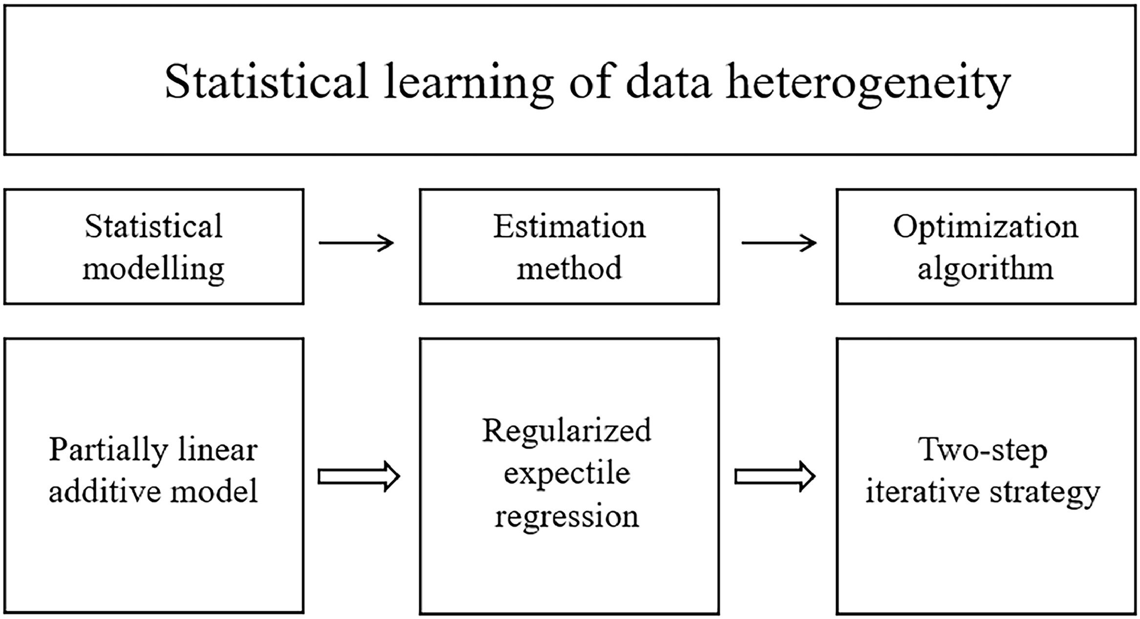
Statistical learning of data heterogeneity

To illustrate the procedure of statistical learning of data heterogeneity more effectively, we accordingly divide the structure of this section into three parts as Fig. 1 presents,

Fig. 1.

The procedure of statistical learning of data heterogeneity.

Statistical modelling: partially linear additive process

Suppose that a high-dimensional data sample {Yi,xi,zi}i=1n is collected, where Yi,i=1,…,n are the response variables, xi=(xi1,…,xip),i=1,…,n are independent and identically distributed p-dimensional covariates along with the common mean 0 and zi=(zi1,…,zid),i=1,…,n are d-dimensional covariates. This paper employs the following popular partially linear additive model for such data,

where g0(zi)=μ0+∑j=1dg0j(zij). It should be noted that our approach to data heterogeneity is inspired by the concept of 'variance heterogeneity' from Rigby and Stasinopoulos (1996)'s mean and dispersion additive model. Specifically, in our modelling, ϵi can be generalized to take the following more general form,

whereσ(xi,zi), conditional onxandz, can be nonconstant, linear form, nonparametric form.

In addition to heterogeneity, {ϵi}i=1n are assumed to be mutually independent.

Estimation method: regularized expectile framework

To deal with data heterogeneity, quantile regression is a common choice for analyzing data heterogeneity in classical statistical estimation method since it can capture the complete conditional distribution of the response variable given the covariates. However, for high-dimensional heterogeneous data, quantile regression faces challenges such as complex optimization algorithms, high computational costs, and difficult statistical inference. This paper employs expectile regression with the asymmetric square loss ϕα(·),

The α-th expectile of random variable Y is defined correspondingly as

Analogue to quantile, expectile can infer the whole conditional distribution of Y.

Before we present our method in detail, let us revisit the popular semiparametric model (2.1). For general statistical modelling, data follow this underlying generation process below. We assume that for some specific α, mα(Y|x,z) has a partially linear additive structure.

Therefore, under mα(ϵi|xi,zi)=0, the conditional α-th expectile ofYessentially satisfies mα(Y|x,z)=μ0+∑k=1pβk*xk+∑j=1dg0j(zj). Thus, β*andg0(·) minimize the following population risk,

For identification purpose, without loss of generality, each g0j is assumed to has zero mean, so that the minimizer (β*,g0(z)) of the population risk is unique.

In this article, the dimensionality of the nonparametric components covariates d is fixed while the covariates x follows high dimensional setting, i.e., p=p(n) is much larger than n and can increase with the sample size n. One way to deal with this high dimension setting is to impose some low-dimensional structure constraints. One leading framework is to assume that the true parameterβ*=(β1*,…,βp*)is sparse. Let A={j:βj*≠0,1≤j≤p} be the active index set of significant variables and q=q(n)=|A|.Without loss of generality, we rewrite β*=((βA*)′,0′)′ where βA*∈Rq and0denotes a(p−q)dimensional vector of zero. The nonparametric components g0j(·),j=1,…,d in model (2.1) are approximated by a linear combination of B-spline basis functions. Let π(t)=(b1(t),…,bkn+l+1(t))′ denote a vector of normalized B-spline basis functions of order l+1 with kn quasi-uniform internal knots on [0,1]. Denote by Π(zi)=(1,π(zi1)′,…,π(zid)′)′, then g0(zi) can be linearly approximated by Π(zi)′ξ, whereξ∈RDn,Dn=d(kn+l+1)+1. Schumaker (2007) have proved that this linear approximation can fit well enough.

Regularized framework has been playing a leading role in analyzing high-dimensional data in recent years. We define the following penalized expectile loss function for our model,

There are different lines of choices for the penalty function Pλ(t) with tuning parameter λ. The L1 penalty or the well-known Lasso is a popular choice for penalized estimation since it induces a convex optimization problem such that it brings convenience in theoretical analysis and computation. However, the L1 penalty is known to over-penalize large coefficients, tends to be biased and requires strong irrepresentable conditions on the design matrix to achieve selection consistency. This is usually not a concern for prediction, but can be undesirable if the goal is to identify the underlying model. In comparison, an appropriate nonconvex penalty function can effectively overcome this problem; see Fan and Li (2001). So throughout this paper, we assume that Pλ(t) is a general folded concave penalty, for examples, the two popular SCAD or MCP penalty;

• •

  The SCAD penalty is defined through its first order derivative and symmetry around the origin. To be specific, for θ>0,

  

where a>2 is a fixed parameter.

• •

  The MCP penalty has the following form:

  

where b>0 is a fixed parameter and sgn(·) is the sign function.

From the definition above, the SCAD or MCP penalty is symmetric,non-convex on [0,∞), and singular at the origin. a=3.7 and b=1 are suggested as a practical choice for the SCAD or MCP penalty respectively for good practical performance in various variable selection problems.

The proposed estimators are obtained by solving the following optimization problem,

Denote by ξ^=(ξ^0,ξ^1,…,ξ^d), then the estimator of g0(zi) is

where

If we could foresee which variables would be significant with divine foreknowledge, this would theoretically yield the best possible statistical analysis outcome, known as the oracle estimator (Fan & Li, 2001). Following their idea, we first introduce the oracle estimator for partially linear additive model (2.1), denoted by(β^*,ξ^*)with β^*=(β^A*′,0p−q)′ through the following optimization problem,

The cardinalityqnof the index set A is allowed to change with n so that a more complex statistical model can be fit when more data are collected. Under some mild conditions, the oracle estimator obtained by the optimization problem (2.5) shares the best estimation accuracy,

The estimation accuracy is influenced by the model size qn since qn is allowed to change with n. In the case qn is fixed, the rates reduce to the classical rate n−1/2 for estimating β and n−2r/(2r+1) for estimating g0(·)for the optimal rate of convergence.

Furthermore, the oracle estimator (β^A*,ξ^*) can be proved as a strict local minimum of the nonconvex optimization problem (2.4). By the constraints on λ, we find out that the error moment and the signal strength directly influence the dimensionality our proposed method can handle. If given the covariates ∈i has all the moments, this asymptotic result holds when p=O(nτ) for any τ>0. What's more, if the error ∈ follows gaussian or sub-gaussian distributions, it can be showed that our method can be applied to ultra-high dimension.

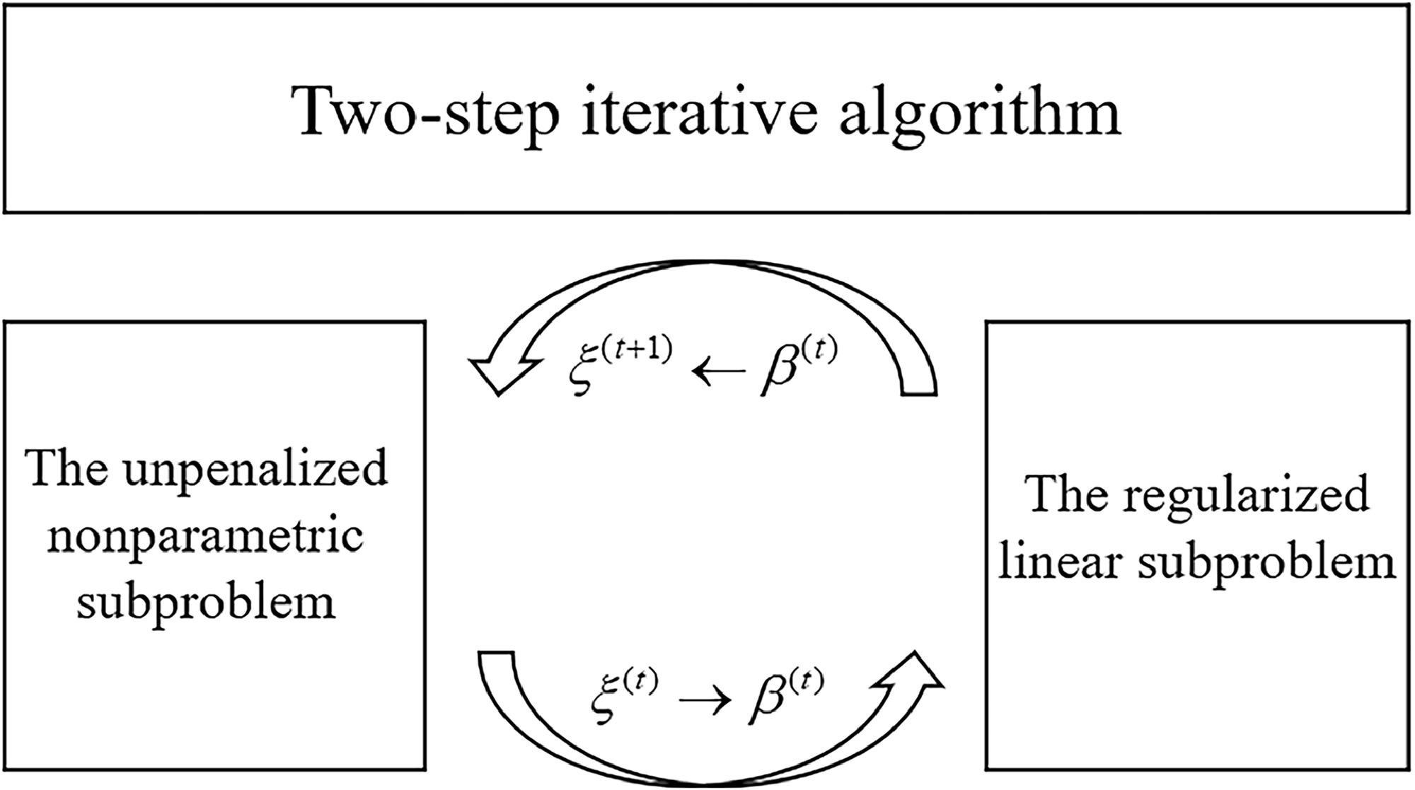
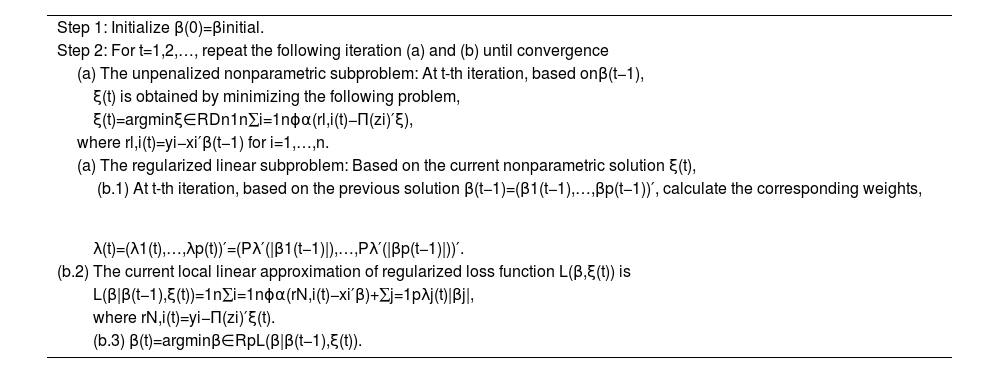
Optimization algorithm: two-step iterative strategy

After the regularized partially linear additive expectile regression is proposed, it is essential to also develop corresponding optimization algorithms. This integration is crucial for transitioning statistical theory into practice. For the optimization problem (2.4), note that there is no penalty on the nonparametric coefficientsξ. So instead of taking (β,ξ) as the whole optimization parameters, we decompose the optimization problem into two subproblems: the fixed dimensional unpenalized nonparametric part and the high dimensional penalized linear part, and propose an iterative two-step algorithm. The iterative updating process for algorithms is shown in Fig. 2. To be specific, in the first step, we obtain the nonlinear part's parameters by minimizing an unpenalized objective function in Dn dimension with the parameters from the linear part valued at its last-iteration result. Note that the expectile loss function ϕα(·) is differentiable and strongly convex by Lemma 1 in Gu and Zou (2016), this optimization problem can be easily done by convex analysis. Then after solving the nonparametric optimization problem, in the second step, we obtain the linear part's parameters by minimizing a penalized expectile loss function. Due to the non-convexity of the penalty Pλ(t), we have to deal with a non-convex optimization problem in high dimension. We take use of the local linear approximation (LLA, Zou & Li, 2008) strategy to approximate it into a sequence of convex ones. The LLA strategy has been proven to enjoy good computational efficiency and statistical properties, see Fan et al. (2014). To sum up, the details are presented in Algorithm 1.

Fig. 2.

The two-step iterative process of our proposed algorithm.

Algorithm 1.

The two-step iterative algorithm for the nonconvex optimization problem (2.4).

Step 1: Initialize β(0)=βinitial.

Step 2: For t=1,2,…, repeat the following iteration (a) and (b) until convergence

(a) The unpenalized nonparametric subproblem: At t-th iteration, based onβ(t−1),

ξ(t) is obtained by minimizing the following problem,

ξ(t)=argminξ∈RDn1n∑i=1nϕα(rl,i(t)−Π(zi)′ξ),

where rl,i(t)=yi−xi′β(t−1) for i=1,…,n.

(a) The regularized linear subproblem: Based on the current nonparametric solution ξ(t),

(b.1) At t-th iteration, based on the previous solution β(t−1)=(β1(t−1),…,βp(t−1))′, calculate the corresponding weights,

λ(t)=(λ1(t),…,λp(t))′=(Pλ′(|β1(t−1)|),…,Pλ′(|βp(t−1)|))′.

(b.2) The current local linear approximation of regularized loss function L(β,ξ(t)) is

L(β|β(t−1),ξ(t))=1n∑i=1nϕα(rN,i(t)−xi′β)+∑j=1pλj(t)|βj|,

where rN,i(t)=yi−Π(zi)′ξ(t).

(b.3) β(t)=argminβ∈RpL(β|β(t−1),ξ(t)).

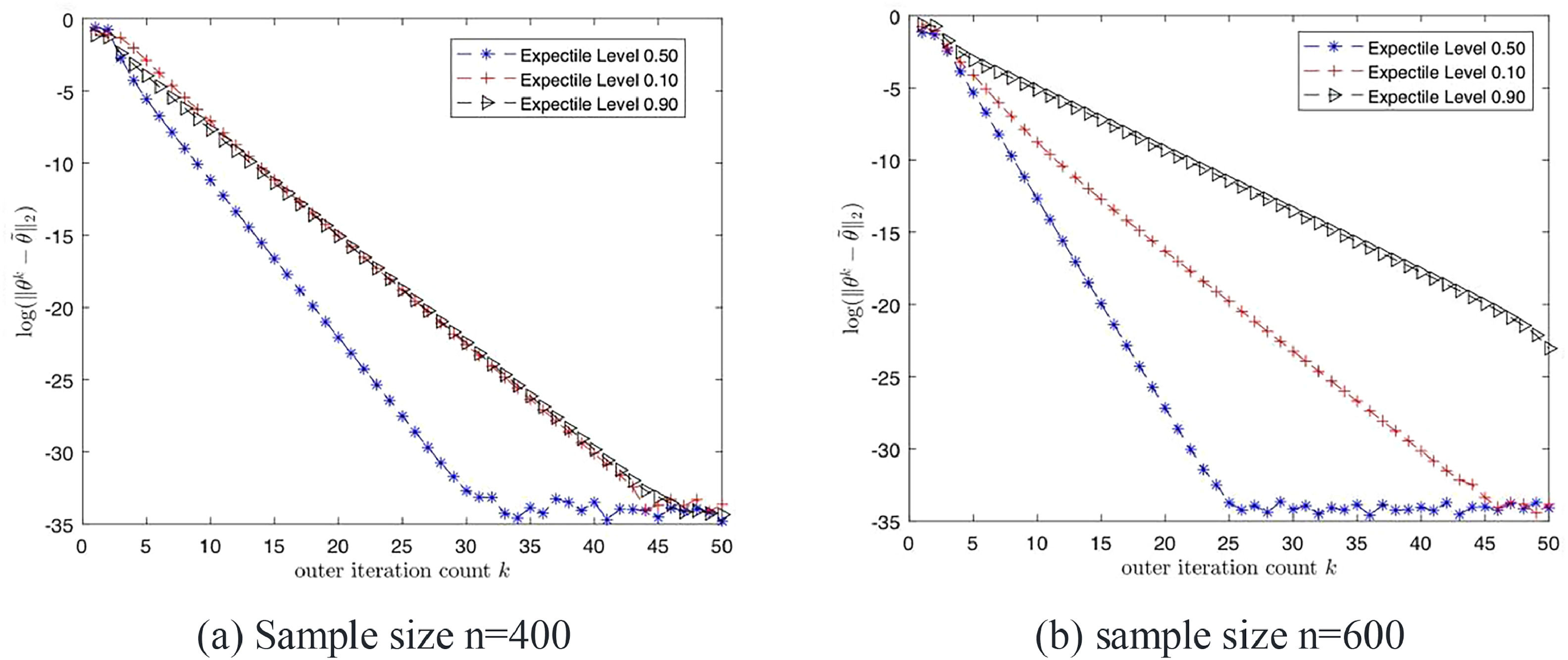
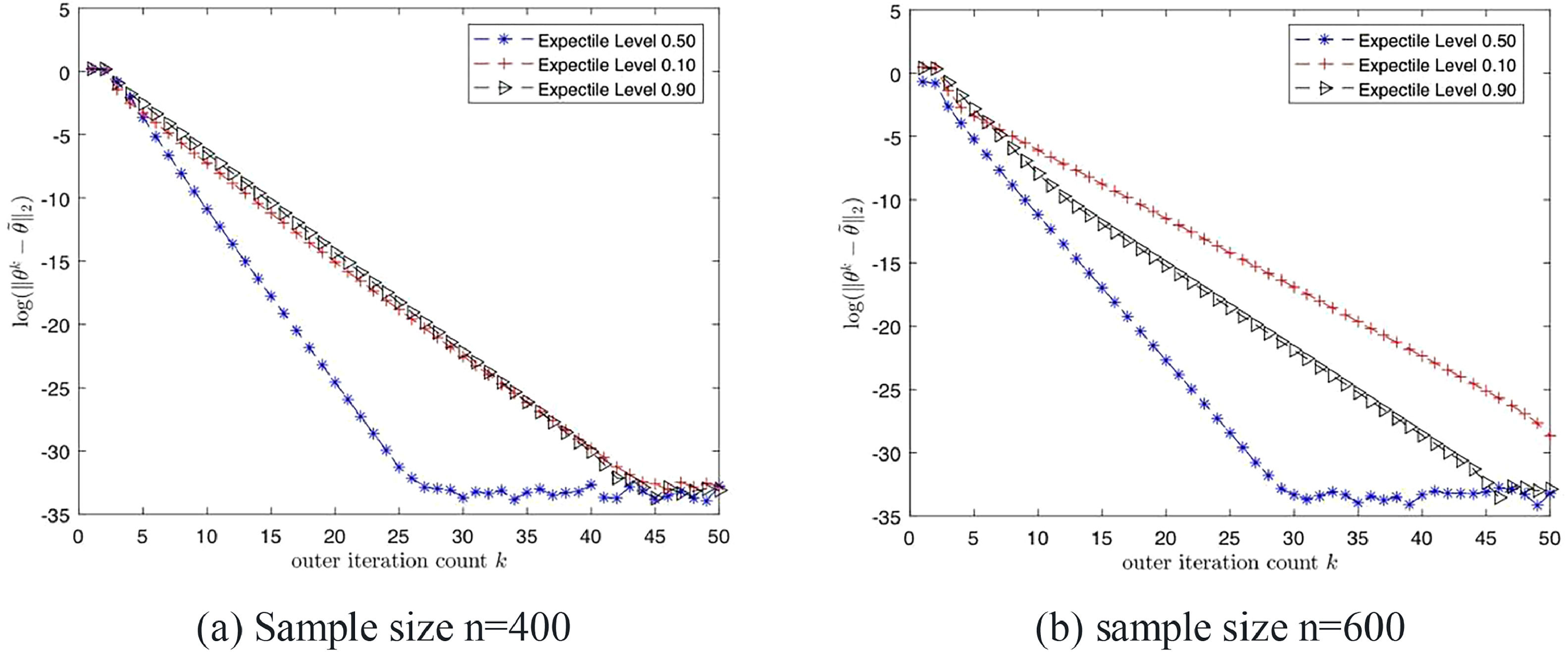
Under some mild conditions, Algorithm 1 initialized by β(0) converges to the oracle estimator (β^*,ξ^*) after a few iterations with the overwhelming probability. What's more, the proposed two-step Algorithm 1 converges at least linearly to the oracle estimator. Fig. 3 and 4 plot log-estimation loss (mean squared error) versus the iteration count in one solution process under the setting in our simulation section, which further demonstrate that the proposed algorithm converges fast and stably.

Fig. 3.

Convergence Rate of Algorithm 1 when ϵ follows t5 Distribution.

Fig. 4.

Convergence Rate of Algorithm 1 when ϵ follows N(0,1) Distribution.

Since the oracle estimator (β^*,ξ^*) is a strict local minima of problem (2.4), it can be expected that this most 'efficient' estimator is available once the iteration solution enters some neighborhood of the oracle estimator. Buhlmann and Van De Geer (2011) suggest that the lasso-type estimator shares good estimation accuracy Op(qnpn). So the initial valueβ(0)can be chosen as the estimator from the following pseudo-linear penalized expectile regression, just ignoring the nonlinear effect,

Furthermore, even the initial value is chosen as the worst case, βinitial=0, through our designed iteration procedure, it is noteworthy that for the next iteration step in the linear subproblem, it is also turned into the lasso-type optimization problem. In a word, our proposed Algorithm 1 is robust to the choice of the initial value βinitial.

Simulation

In this section, we assess the finite sample performances of our proposed regularized expectile regression in coefficients estimation, nonparametric approximation and model identification in high dimension. For the choice of the general folded concave penalty function Pλ(t), here we use the SCAD penalty as an example. For convenience, denote the penalized partially linear additive expectile regression with the SCAD penalty by E-SCAD for short. For comparative purpose, in this simulation, we also investigate the performance of the Lasso-type regularized expectile regression (E-Lasso for short). One may use L1-penalty instead of SCAD penalty in penalized expectile regression and solve the following optimization problem,

We aim to show the differences when we use L1-penalty or the SCAD penalty in regularized expectile regression and furthermore tell the reason why we choose the SCAD penalty instead of L1-penalty in this article. Besides, for comparison benchmark, we introduce the oracle estimator as the benchmark of estimation accuracy.

We adopt a high-dimensional partially linear additive model from Sherwood and Wang (2016). In this data generation process, firstly, the quasi-covariates x~=(x~1,…,x~p+2)′ is generated from the multivariate normal distribution Np+2(0,Σ) where Σ=(σij)(p+2)×(p+2), σij=0.5|i−j| for i,j=1,…,p+2. Then we set x1=12Φ(x~1) where Φ(·) is the cumulative distribution function of the standard normal distribution and 12 scales x1 to have standard deviation 1. Furthermore, let z1=Φ(x~25) and z2=Φ(x~26), xi=x~i for i=2,…,24 and xi=x~i+2 for i=25,…,p. Then the response variable y is generated from the following sparse model,

where βj=1 for j=6,12,15,20 and ϵ is independent of the covariates x.

Now let us focus our attention to the heterogeneous case. Here we assume the heteroscedastic structure ϵ=0.70x1ς, where ς is independent of x1 and follows the N(0,1) or t5. In this heterogeneous situation, x1 should also be regarded as the significant variable since it plays an essential role in the conditional distribution of y given the covariates and results in heteroscedasticity. So besides parameter estimation and model selection, we also want to test whether our proposed method can be used to identify x1 and detect heteroscedasticity.

We set sample size n=300 and covariate dimension p=400 or 600. For expectile weight level, by the results in Newey and Powell (1987), positions near the tail seem to be more effective for testing heteroscedasticity, so we consider two positions: α=0.10,0.90. Note that when α=0.50, expectile regression is exactly the classical ordinary least squares regression, so we also consider the position α=0.50 so as to show our proposed method can be used to detect heteroscedasticity when α≠0.50. Given the expectile weight level α, there are two tuning parameters in SCAD penalty function, a and λ. We follow the suggestion proposed by Fan and Li(2001) and set a=3.7 to reduce the computation burden. For the tuning parameter λ, we generate another tuning data set with size 10n and choose the λ that minimizes the prediction expectile loss error calculated on the tuning data set. Other information criteria to determine the tuning parameter λ can be found in Wu and Wang (2020). For the nonparametric components, we adopt the cubic B-spline with 3 basis functions for each nonparametric function.

We repeat the simulation procedure 100 times and report the performances in terms of the following criteria:

• •

  AE: the absolute estimation error defined by ∑ip|β^j−βj*|.

• •

  SE: the square estimation error defined by ∑ip|β^j−βj*|2.

• •

  ADE: the average absolute deviation of the fit of the nonlinear part defined by 1n∑i=1n|g^(zi)−g0(zi)|

• •

  Size: the number of nonzero regression coefficients β^j≠0 for j=1,…,p. In the heteroscedastic case, given the role of x1, the true size of our data generation model supposes to be 5.

• •

  F: the frequency that x6,x12,x15,x20 are selected during the 100 repetitions.

• •

  F1: In the heteroscedastic case, the frequency that x1 is selected during the 100 repetitions.

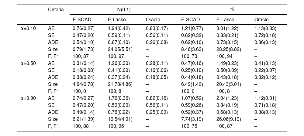
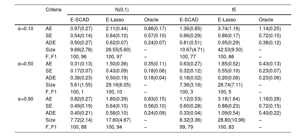
Table 1 presents the average performance of these methods based on 100 repeated simulations in high-dimensional heterogeneous data. These include AE, SE, and ADE as three indicators to evaluate the model's statistical analysis accuracy. It is evident that E-SCAD exhibits smaller errors compared to E-Lasso. Compared to the Oracle estimator, E-SCAD more closely approximates its performance and tends toward theoretically optimal estimation accuracy. Size, F, and F1 are indicators used to assess variable selection and heterogeneity identification performance in the model. According to the SIZE indicator, E-SCAD tends to select a number of variables closer to the true model size. Although the frequency of F1 is relatively lower, it is achieved at a smaller model size. Therefore, we can conclude that overall, E-SCAD demonstrates significantly better estimation accuracy than E-Lasso, as illustrated in Table 1. In Table 2, we expanded the data dimensions in our simulation settings from 400 to 600, leading to similar conclusions. So, we may tend to use the SCAD penalty instead of the Lasso penalty in practice. Besides, first note that in our simulation setting mα=0.5(ϵ|x,z)=0, then at this moment, E-SCAD has better performances in estimation accuracy and model selection than those with other weight levels α=0.1,0.9, confirmed by the AE, ADE and SE results. However, the variance heterogeneity does not show up in mα=0.50(y|x,z) so that at this situation E-SCAD cannot pick x1, the active variable resulting in heteroscedasticity. Expectile regression with different weights can actually help solve this problem. We can see that at α=0.1 and α=0.90, x1 can be identified as the active variable with high frequency. On the other hand, from Table 1 to Table 2, as p increases, we can see that the performances of E-SCAD get a little worse, and this change is more obvious in t5 case. We have to say that the dimensionality our proposed method can handle is influenced by the heavy-tailed characteristics of the error. Our theoretical study indicates that if the regression error has only finite moments like in the t5 case, pcan be at most a certain power of n.

Table 1.

Simulation results for heteroscedastic errors when n=300, p=400.

	Criteria	N(0,1)			t5
		E-SCAD	E-Lasso	Oracle	E-SCAD	E-Lasso	Oracle
α=0.10	AE	0.76(0.27)	1.94(0.42)	0.83(0.17)	1.21(0.77)	3.01(1.22)	1.13(0.33)
	SE	0.47(0.20)	0.59(0.11)	0.56(0.11)	0.62(0.32)	0.83(0.21)	0.72(0.18)
	ADE	0.54(0.10)	0.67(0.10)	0.26(0.08)	0.62(0.10)	0.73(0.15)	0.36(0.13)
	Size	6.79(1.73)	24.05(5.51)	–	8.46(3.63)	28.25(8.82)	–
	F, F1	100, 87	100, 97	–	100, 73	100, 94	–
α=0.50	AE	0.31(0.14)	1.26(0.30)	0.28(0.11)	0.47(0.16)	1.49(0.23)	0.41(0.13)
	SE	0.18(0.08)	0.41(0.09)	0.16(0.06)	0.25(0.10)	0.50(0.09)	0.22(0.07)
	ADE	0.38(0.24)	0.37(0.24)	0.18(0.05)	0.44(0.18)	0.43(0.18)	0.32(0.12)
	Size	4.64(0.78)	21.78(4.86)	–	6.49(1.42)	20.43(3.01)	–
	F, F1	100, 0	100, 8	–	100, 0	100, 8	–
α=0.90	AE	0.74(0.27)	1.76(0.36)	0.82(0.16)	1.07(0.52)	2.94(1.23)	1.12(0.31)
	SE	0.47(0.20)	0.59(0.09)	0.56(0.11)	0.59(0.26)	0.84(0.19)	0.71(0.18)
	ADE	0.49(0.14)	0.76(0.22)	0.25(0.09)	0.52(0.37)	0.68(0.13)	0.38(0.13)
	Size	6.21(1.39)	19.54(4.91)	–	7.74(3.19)	26.06(9.19)	–
	F, F1	100, 88	100, 96	–	100, 76	100, 87	–

Note: Standard deviation error in parentheses based on 100 repetitions.

Table 2.

Simulation results for heteroscedastic errors when n=300, p=600.

	Criteria	N(0,1)			t5
		E-SCAD	E-Lasso	Oracle	E-SCAD	E-Lasso	Oracle
α=0.10	AE	0.97(0.27)	2.11(0.44)	0.86(0.17)	1.36(0.85)	3.74(1.16)	1.14(0.25)
	SE	0.54(0.14)	0.64(0.10)	0.57(0.10)	0.66(0.29)	0.86(0.17)	0.72(0.15)
	ADE	0.50(0.27)	0.62(0.07)	0.24(0.07)	0.81(0.51)	0.95(0.29)	0.38(0.12)
	Size	9.68(2,78)	26.55(5.60)	–	10.67(4.71)	42.53(9.50)	–
	F, F1	100, 96	100, 97	–	100, 77	100, 86	–
α=0.50	AE	0.31(0.13)	1.50(0.36)	0.35(0.11)	0.63(0.27)	1.85(0.52)	0.43(0.13)
	SE	0.17(0.07)	0.43(0.09)	0.18(0.06)	0.32(0.12)	0.55(0.10)	0.23(0.07)
	ADE	0.38(0.23)	0.50(0.19)	0.18(0.04)	0.18(0.02)	0.20(0.06)	0.23(0.06)
	Size	5.61(1.55)	29.16(6.05)	–	7.36(3.16)	26.74(7.11)	–
	F, F1	100, 1	100, 10	–	100, 3	100, 5	–
α=0.90	AE	0.82(0.27)	1.80(0.39)	0.83(0.15)	1.12(0.53)	3.18(1.64)	1.16(0.28)
	SE	0.49(0.19)	0.64(0.10)	0.56(0.10)	0.60(0.28)	0.88(0.23)	0.72(0.15)
	ADE	0.40(0.21)	0.58(0.10)	0.24(0.09)	0.33(0.04)	1.09(0.54)	0.40(0.22)
	Size	7.72(2.14)	17.60(4.67)	–	8.32(3.36)	28.80(10.98)	–
	F, F1	100, 88	100, 94	–	99, 79	100, 83	–

Note: Standard deviation error in parentheses based on 100 repetitions.

Real data application

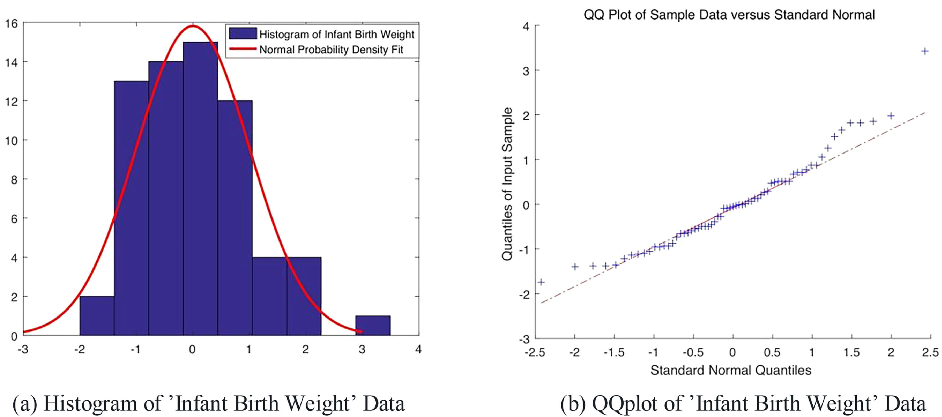
Low infant birth weight has always been a comprehensive quantitative trait, as it affects directly the post-neonatal mortality, infant and childhood morbidity, as well as its life-long body condition. Thus, on purpose of public health intervention, scientists have long put considerable investigation onto the low birth weight's determinants, see Kramer (1987), who investigated 43 potential determinants and used a set of priori methodological standards to assess the existence and magnitude of the effect from potential factor to low birth weight. Turan et al. (2012) used gene promoter-specific DNA methylation levels to identify genes correlated to low birth weight, with cord blood and placenta samples collected from each newborn. Votavova et al. (2011) collected samples of peripheral blood, placenta and cord blood from pregnant smokers (n=20) and gravidas (n=52) without significant exposure to cigarettes smoke. Their purpose was to identify the tobacco smoke-related defects, specifically, the transcriptome alterations of genes induced by the smoke. As the infant's birth weight was recorded along with the age of mother, gestational age, parity, maternal blood cotinine level and mother's BMI index, we consider using this data set to depict the infant birth weight's determinants. The dataset is publicly available at the NCBI Gene Expression Omnibus data repository¹under accession number GSE27272. With a total of 65 observations contained in this genetic set, the gene expression profiles were assayed by Illumina Expression Beadchip v3 for the 24,526 gene transcripts and then normalized in a quantile method. Fig. 5 displays the histogram and QQ-plot of the infant birth weight data. Intuitively, it appears to belong to the normal distribution family. For a more accurate evaluation, we apply Lilliefors Test to the infant birth weight data and the result further confirms our judgement at the default 5 % significance level.

Fig. 5.

Graphical view of 'infant birth weight' data.

To investigate the low birth weight of infant, we apply our partially linear additive penalized expectile regression model into this data set. We consider to include the normalized genetic data, clinic variables parity, gestational age, maternal blood cotinine level and BMI as part of the linear covariates. And we take the age of mother as the nonparametric part to help explain nonlinear effect, according to Votavova et al. (2011). For sake of the possibly existing heteroscedasticity of these data and to dissect the cause of low infant birth weight, the analysis is carried out under three different expectile levels 0.10, 0.30 and 0.50. And in each scenario, feature screening methods could be used to select the top 200 relevant gene probes, see He et al. (2013). Here in our data analysis, we choose to use the SCAD penalty in our regularized framework and denote it by E-SCAD for short. Other nonconvex penalties like MCP penalty could also be applied with our model, for which we don't give unnecessary details. For comparison purpose, we also consider penalized semiparametric regression withL1norm penalty, i.e., the Lasso-type regularized framework, named as E-Lasso. As recommended, the parameter a in the SCAD penalty is set to be 3.7 in order to reduce computation burden. As for the tuning parameter λ, here we adopt the five-folded cross validation strategy to determine its value for both E-SCAD and E-Lasso.

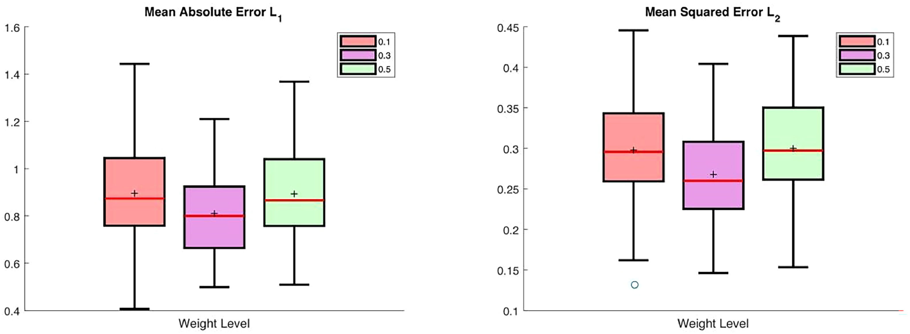
First, we apply our proposed E-SCAD method to the whole data at three different expectile levels α= 0.1, 0.3and 0.5. And for each level, the set of selected variables in the linear part of our model is denoted by A^α, along with its cardinality |A^α|. Taking the possibly existing heteroscedasticity into consideration, we also display the number of overlapped selected variables under different expectile levels, denoted by |A^0.1∩A^0.5| and |A^0.3∩A^0.5|. The number of selected variables and overlapped variables are reported in Table 3. Next, we randomly partition the whole data set into a training data set of size 50 and a test set of size 15. E-SCAD or E-Lasso is applied to the training set to obtain regression coefficients and nonparametric approximation. Then the estimated model is used to predict the responses of 15 individuals in the test set. We repeat the random splitting process 100 times. The variable selection results under random partition scenario are also shown in Table 3. We also report the average absolute error L1 and the average squared error L2 for prediction evaluation. Also, a boxplot of both two prediction evaluation criteria is displayed in Fig. 6. As shown in Table 3 and Fig. 6, the underlying models selected under three expectile levels α=0.1,0.3,0.5 all lead to a relatively small prediction error. In Table 3, the selected genes and corresponding cardinalities are different for different weight levels, which means that different levels of birth weight are influenced by different genes, an indication of heterogeneity in the data.

Table 3.

Summary of proposed method at three different expectile levels.

	Criteria	α=0.1		α=0.3		α=0.5
		E-SCAD	E-LASSO	E-SCAD	E-LASSO	E-SCAD	E-LASSO
All Data	L1	0.66	0.67	0.60	0.53	0.38	0.34
	L2	0.12	0.11	0.10	0.09	0.06	0.05
	A^α	7.00	8.00	9.00	19.00	14.00	20.00
	A^α∩A^0.5	1	1	3	3	–	–
Randon Partition	L1	0.90(0.21)	0.74(0.17)	0.81(0.17)	0.59(0.13)	0.89(0.20)	0.41(0.08)
	L2	0.30(0.07)	0.26(0.06)	0.27(0.06)	0.19(0.04)	0.30(0.06)	0.13(0.02)
	A^α	5.72(1.91)	8.19(2.74)	9.00(2.72)	13.94(3.03)	4.72(1.83)	20.25(2.67)
	A^α∩A^0.5	3.86(1.6433)	1.16(0.39)	2.27(1.13)	3.25(1.18)	–	–

Fig. 6.

Boxplots of prediction errors under different expectile levels.

Table 4 tells us more about data heterogeneity and provides possible guidance for public health intervention. Gestational age is the most frequently selected covariate under all three scenarios, explaining the known fact that premature birth is usually accompanied by low birth weight. Besides, SLCO1A2, LEO1, FXR1 and GPR50 appear frequently in all three cases. Furthermore, an interesting observation arises that the scenarios α=0.1 and α=0.5 perform similarly while the scenario α=0.3 displays some different characteristics. Gene SLCO1A2 is selected with higher frequencies when α=0.1 and α=0.5. This gene is known to have resistance against drug use and moreover, according to Votavova et al. (2011), exposure to toxic compounds contained in tobacco smoke can be strongly associated with low birth weight. Gene EPHA3 is more frequently selected under the scenario α=0.3 compared with other two cases. As shown in Lv et al. (2018), EPHA3 is likely to contribute tumor growth in human cancer cells, which may make pregnant women more sensitive to chemical compounds contained in cigarette smoke. And the study of Kudo et al.(2005) concludes that EPHA3′s expression at both the mRNA and protein level is a critical issue during mammalian newborn forebrain's development. These results can well account for our analysis under different expectile values and may furthermore, arise more our attention upon the α=0.3 expectile value case, due to its specially selected results and potentially underlying biomedical meaning.

Table 4.

Top 6 frequent covariates selected at three expectile levels among 100 partitions.

E−SCADα=0.1		E−SCADα=0.3		E−SCADα=0.5
Variables	Frequency	Variables	Frequency	Variables	Frequency
PTPN3	34	GPR50	46	PTPN3	33
FXR1	40	FXR1	49	GPR50	40
GPR50	43	EPHA3	50	FXR1	41
LEO1	43	LEO1	59	LEO1	44
SLCO1A2	63	LOC388886	65	SLCO1A2	65
Gestational age	79	Gestational age	97	Gestational age	83

Discussion

In this paper, we propose a flexible regularized partially linear additive expectile regression with general nonconvex penalties for high-dimensional heterogeneous data. We take full advantages of expectile regression in computation and analysis of heterogeneity, and propose a fast and stable two-step algorithm for the induced optimization problem. In our framework, we make two main contributions. First of all, unlike most existing works assume errors follow Gaussian or sub-Gaussian distributions, we make a less stringent and more realistic assumption that the errors only have finite moments. Under this general condition, we show theoretically that the oracle estimator is a strict local minimum of our optimization problem. The other contribution is that we derive a two-step algorithm to solve the nonconvex and nonsmooth problem (2.4), and we show that the proposed algorithm converges at least linearly. Monte Carlo simulation studies and real data application indicate that our proposed method enjoys good performances in estimation accuracy, nonparametric approximation and model selection, especially heterogeneity identification. These two contributions make the proposed partially linear additive regularized expectile regression an alternative choice to statistical learning of high-dimensional heterogeneous data.

Our theoretical result implies that the dimensionality our proposed method can handle is influenced by the moment order the error has. This polynomial relation between n and p may restrict our method not available to the ultrahigh dimensional setting (log(p)=O(nb),0

In the model build-up process, a problem of important practical interest is how to identify which covariates should be modeled linearly and which covariates should be modeled nonlinearly. In our real data application section, we distinguish these two parts according to our experience and the existing result. This challenging problem involves goodness-of-fit of our model. Expectile can draw a complete picture of the conditional distribution given the covariates, which provides a potential way to solve this problem. We plan on addressing this question for high dimensional semiparametric expectile regression in our future research.

CRediT authorship contribution statement

Jun Zhao: Writing – review & editing, Writing – original draft, Methodology, Data curation, Conceptualization. Fangyi Lao: Data curation, Visualization. Guan'ao Yan: Software, Resources, Methodology. Yi Zhang: Methodology, Formal analysis, Conceptualization.

CRediT authorship contribution statement

Jun Zhao: Writing – review & editing, Writing – original draft, Methodology, Data curation, Conceptualization. Fangyi Lao: Data curation, Visualization. Guan'ao Yan: Software, Resources, Methodology. Yi Zhang: Methodology, Formal analysis, Conceptualization.

Acknowledgements

Jun Zhao thanks support from the MOEProject of Humanities and Social Sciences of China (No. 21YJCZH235), the Hangzhou Joint Fund of the Zhejiang Provincial Natural Science Foundation of China under Grant No. LHZY24A010002 and Scientific Research Foundation of Hangzhou City University (No. J-202315).