Single Maneuvering Target Tracking in Clutter Based on Multiple Model Algorithm with Gaussian Mixture Reduction

Abstract

The measurement origin uncertainty and target (dynamic or/and measurement) model uncertainty are two fundamental problems in maneuvering target tracking in clutter. The multiple hypothesis tracker (MHT) and multiple model (MM) algorithm are two well-known methods dealing with these two problems, respectively. In this work, we address the problem of single maneuvering target tracking in clutter by combing MHT and MM based on the Gaussian mixture reduction (GMR). Different ways of combinations of MHT and MM for this purpose were available in previous studies, but in heuristic manners. The GMR is adopted because it provides a theoretically appealing way to reduce the exponentially increasing numbers of measurement association possibilities and target model trajectories. The superior performance of our method, comparing with the existing IMM+PDA and IMM+MHT algorithms, is demonstrated by the results of Monte Carlo simulation.

1

Introduction

Two difficulties arise in the problem of single maneuvering target tracking in clutter: target (dynamic or/and measurement) model uncertainty and measurement origin uncertainty. Algorithms dealing with these two problems individually abound in previous studies [1–6].

First, target maneuvers incur target dynamic model uncertainty in tracking. The multiple model (MM) algorithms [6–9] were proposed and have been gaining prevalence to address this problem. Instead of modeling a target motion by a single dynamic model, a set of models are implemented in parallel in MM and the result is computed based on the outputs from all of these models.

Second, measurement origin uncertainty arises when false measurements (measurements not originated from a target) are received in a sensor scan. Many factors could contribute to the reception of false measurements. For example, clutter, thermal noise, electronic counter-measurements, so on and so forth. The multiple-hypothesis tracker (MHT) [4, 10–15] is a powerful tool for this problem. It branches all possible (or several most probable) association hypotheses and the tracking result is obtained based on the results of all available hypotheses.

One similarity between MM and MHT is that their optimal implementations require exponentially increasing numbers of model sequences and hypotheses respectively, which make their optimal solutions infeasible in practice. In this work, MHT and MM are combined, and the numbers of model sequences and hypotheses are reduced in a joint way based on the Gaussian mixture reduction (GMR) [16–22]. Combinations of MHT and MM, especially the interacting-multiple model (IMM), were proposed in previous studies, but, in a straightforward and somewhat crude manner. That is, the two algorithms were simply put together to tackle the two problems one at a time and each algorithm functions separately without exploring the connection to the other one and to the mutual effects on the final performance. We propose the reduction based on GMR, which provides a more solid and appealing way than existing methods to reduce jointly the numbers of model sequences and hypotheses. The density of a target state is a Gaussian mixture with each component corresponding to a model sequence and a hypothesis (under a linear Gaussian assumption). In our method, the number of Gaussian components is reduced by merging the “similar” ones, which are selected by a “distance” defined between two Gaussian components. Clearly, our method does a joint reduction instead of reducing the numbers of model sequences and hypotheses separately. Furthermore, GMR attempts to minimize the impact of merging to the original Gaussian mixture, which is theoretically more solid and better justified than conventional methods, e.g., GPBn or IMM. The superior performance of our method is demonstrated by the results of Monte Carlo simulation by comparing with the existing IMM+PDA and IMM+MHT algorithms.

This paper is organized as follows. The problem of single maneuvering target tracking in clutter is formulated in Section 2. The Gaussian mixture reduction is elaborated in Section 3. Multiple mode algorithm based on Gaussian mixture reduction is presented in Section 4 and its combination with MHT is given in Section 5. Numerical examples are given in Section 6 and conclusion remarks are made in Section 7.

2

Problem formulation

We consider the problem of single maneuvering target tracking in clutter, that is, we assume that only one target is presented in the surveillance region and it has the following first-order Markov jump linear motion models

and the measurement model is

Where p = 1,…,m, and m are the index and total number of motion models, respectively, wkp and ν_k are mutually uncorrelated zero-mean white Gaussian noise sequences with covariances QKP and R_k, respectively, and are independent of the initial target state. Denote π(q,p)=Pmkp|mk−1p as the model transition probability, where mkp is the event that the pth model is in effect at time k. The model uncertainty problem must be addressed in a tracking algorithm because in most applications (except for a cooperative target) we are not certain which model is in effect at each time k. The prevailing method is MM [6].

Furthermore, false measurements from clutter or thermal noise may present in each sensor scan. That is, multiple measurements may be received at each sensor scan, rendering their origins uncertain. Most target tracking algorithms dealing with clutter need to address this data association problem explicitly, for example, the nearest or strongest neighbor filter [23–25], probabilistic data association filter [26] and the more powerful (of course, more complicated) multiple hypothesis tracker (MHT) [10,11]. In this work, it is assumed that: a) all the measurements are independent; b) false measurements are also independent to the target state: c) one and only one measurement is originated from a target.

Combinations of MM and data association algorithms to deal with maneuvering target tracking in clutter exist. However, for most cases they were combined in rather heuristic ways that their connections and their mutual effects on the final performance are not explored. In this work, we propose an algorithm based on MM and MHT, where they are integrated by Gaussian mixture reduction.

3

Gaussian mixture reduction

Approximating a Gaussian mixture density with another Gaussian mixture density of a reduced number of components by minimizing the “approximation error” in some sense leads to the Gaussian mixture reduction (GMR) problem [16–22]. Constraints, for example, maintaining the grand mean and covariance, may be further imposed to the problem. The optimal solution may be obtained by solving a high dimensional constrained nonlinear optimization problem which is mathematically intractable for most applications. Rather than direct search of Gaussian componentsfor the reduced mixture, the approximation can be obtained by merging the components in the original mixture. Components to be merged are selected based on their “distance”, to be defined. However, this is actually equivalent to an assignment problem, which is NP hard. Note that even if the optimal merging is achieved, it is not necessary the optimal solution to the GMR problem in general, because the Gaussian components in the optimal solution may not be able to be obtained by merging.

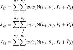
There were many distances proposed for two Gaussian components. They can be categorized into two classes: global distance and local distance. Denote f(x) the original Gaussian mixture density, and f_ij(x) the reduced Gaussian mixture density by merging the ith and jth components. Then, the global distances of components i and j in a mixture are defined by the difference between the densities f(x) and f_ij(x), while local distances are defined in terms of the difference between the two Gaussian components. The global distance is preferred for GMR problem because it considers the overall performance of merging. The PDF correlation coefficient is a distance like measures widely used in statistics [27,28]. The Kullback-Leibler (KL) divergence may be another option [21], but they cannot be evaluated analytically between two Gaussian mixtures, see [29] and reference therein for some numerical methods. Runnalls [21] proposed an upper bound of KL divergence to serve as a distance which is, however, a local one. We adopt the distance proposed by Williams and Mayback [18,19]—the integral squared difference (ISD), which can be analytically evaluated between two Gaussian mixture densities f(x) and g(x). The ISD is defined as

It is a global distance and can be evaluated analytically between any two Gaussian mixture densities:

Where

and {w_i,μ_i,P_i} and w¯i,μ¯i,P¯i are the weights, means and covariances of the ith Gaussian components in f(x) and g(x), respectively. Efficient algorithms to compute the distance were proposed in [19].

Once the distance between Gaussian components is defined, “close” components should be merged. For n Gaussian components with weights w_i, means μ_i and covariance P_i they are merged by

Therefore, the grand mean and covariance are preserved. As mentioned before, optimal merging is difficult to achieve, hence, many efficient suboptimal procedures were proposed. The top-down reduction algorithms based on greedy methods were proposed in [18,19,21], where two of the components are selected to merge at each iteration. The iteration stops until the number of components reduces to a threshold M. Besides, the reduction algorithm based on clustering was proposed in [30]. The dissimilarity matrix, which contains pairwise distances between any two components, is computed and all Gaussian components are clustered into M clusters. The components in the same cluster are merged. Different clustering algorithms [30–32] (e.g., k-means, k-medoids, hierarchical clustering, etc.) are optional.

4

Multiple model algorithm based on Gaussian mixture reduction

First, we elaborate the MM algorithm based on GMR. As explained in the next section, it can be readily extended to incorporate the MHT. The optimal MM has to consider all the possible model trajectories, which is infeasible in practice due to the combinatorial explosion. Many algorithms were proposed to reduce the number of model trajectories [6]. They can be classified as: a) methods based on hard decision, such as the B-Best algorithm, which keeps the most probable one or a few model sequences and prunes the rest; b) methods based on soft decision, such as the GPBn algorithm, which merges those sequences with common model trajectories in the last n steps. In general, the algorithms based on soft decision outperform those based on hard decision. However, in GPBn there is no solid ground to justify why sequences with some common parts should be merged. These common histories do not necessarily make the resulting Gaussian components being “close” to each other. Consequently, the merging may not lead to a good performance. Comparing with the merging methods in GPBn or IMM, the MM based on GMR [18] is better justified—the Gaussian components with “small distance”, rather than “similar model trajectory”, are combined. Although the reduction procedures elaborated in the previous section do not merge the Gaussian components optimally, it is suffice to rely on these suboptimal but efficient procedures to achieve a better performance than the existing methods. The idea is straightforward. All the combinations of Gaussian components up to time k-1 and m system models at time k are considered, resulting in a larger set of Gaussian components. Then, GMR is used to reduce the number of components to a pre-specified number M. One cycle of MM based GMR is given below:

• (1).

  Assume the Gaussian mixture density of target state at k-1 is

  

  Meaning that there are M Gaussian components

  
  with the weights w⌣k−1j. x⌢k−1j and Pk−1j are the state estimate and its MSE matrix respectively, in the jth Gaussian component. Assume the component-to-model transition probability Pmkp|Nk−1j at k-1 is available (computation of this probability is given in step 6).

• (2).

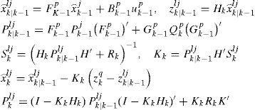
  Model conditional filtering at time k:

  Denote Cki the ith event in the set mkp,Nk−1jj=1,…,Mp=1,…m. Then the conditional posterior density f(xk|Cki,Zk) can be computed by Bayesian rule. For a linear Gaussian system (conditioned on a model sequence), Kalman filter applies. Clearly, there are mM different events Cki and each f(xk|Cki,Zk) is Gaussian distributed.

• (3).

  Component probability update:

  For each Cki, its posterior probability is updated by

  

  Where

  

  Note that as mentioned in Step 1, P{mkp|Nk−1j} is computed at time k-1.

• (4).

  Gaussian mixture reduction:

  Reduce the Gaussian mixture

  
  to a mixture with M components based on a GMR procedure elaborated in the previous section, that is,
  

  Because Nkj is obtained by merging the Gaussian components corresponding to some Cki, an m × 1 auxiliary vector aki is constructed for each Nkj to record the weight (or portion) of each model mkp in Nkj, that is,

  

  Where l(⋅) is the indicator function. Note that unlike GPBn method, after merging, each component Nkj does not have a clear physical meaning.

• (5).

  Estimation fusion:

  The overall density of target state is

  

• (6).

  component-to-model transition probability:

  

  Where π(p,:) is the pth row of the transition probability matrix π and akj=[akj(1),…,akj(m)]′.

• (7).

  k = k + 1 and loop to Step 2.

  If dealing with a nonlinear system, each conditional density f(xk|Cki,Zk) can be approximated by a moment matching Gaussian density, similar as the Gaussian filter [33] does. Although the GMR algorithms do not reduce the Gaussian mixture optimally, they are based on a more solid guideline for merging than the GPBn methods, hence should result in better performance.

5

Combining MM and MHT based on GMR

Similar to MM, which was proposed to address the problem of target model uncertainty, MHT was proposed [10, 11] to address the problem of measurement origin uncertainty for single or multiple targets tracking in clutter.

The MHT is a multi-scan association method. For simplicity, we assume: a) perfect detection probability, i.e., Pd = 1 (for Pd < 1, all the derivation follows similarly but more tedious); b) each measurement only has one source (either the target or clutter) and one target can at most generate one measurement; c) the clutter and true target measurement are independent. Based on these assumptions, MHT generates and propagates hypotheses Hki. Each hypothesis specifies one possible association between the measurements Z^k = {z₁,…,z_k} and the target, where zk={zk1,zk2,…,zkmkz}, and mkz is the total (validated) number of measurements at scan k. For single target tracking, each zkj leads to two association possibilities:

• a)

  It is a continuation of the existing track.

• b)

  It is from clutter.

Similar to MM algorithm, the combinatorial explosion must be addressed to make the MHT practical. Denote hkq the event that zkq is associated to the target at time k. Actually the MHT for single target tracking can be viewed as a MM algorithm. At each sensor scan, each hkq can be viewed as a “model”. Note that the number of the “models” depends on actual number of measurements at each scan k. Validation gate may be applied to reduce the number of false measurements. Combing with Hk−1i, new set of hypotheses {hkq,Hk−1j}j=1,…,mk−1Hq=1,…mkz are generated and they specify all the association histories up to time k, analogous to the model trajectories in MM algorithm.

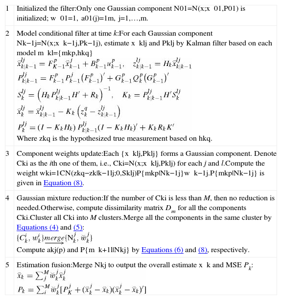
The MM method based on GMR can be directly extended to deal with clutter. The resulting algorithm is denoted as MMG (MM-MHT based on GMR). Based on each motion model mkp and each association event hkq, a set of new “models” can be generated {m⌣kl}={mkp,hkq}p=1,…,mq=1,…,mkz at time k. The MM algorithm in previous section can be directly applied with only minor modifications. First, the model transition probability π is replaced by

Where the assumption that the target model and association event are conditionally independent is made. Second, the likelihood function becomes

Where C is a constant which depends on the clutter density, and zkq is the hypothesized true measurement. A detailed algorithm for a linear Gaussian system with first-order Markovian model jumps is given in Table 1.

Table 1.

Algorithm of MM-MHT based on GMR.

1	Initialized the filter:Only one Gaussian component N01=N(x;x⌢01,P01) is initialized; w⌣01=1,  a01(j)=1m,  j=1,…,m.
2	Model conditional filter at time k:For each Gaussian component Nk−1j=N(x;x⌢k−1j,Pk−1j), estimate x⌢klj and Pklj by Kalman filter based on each model m⌣kl={mkp,hkq} Where zkq is the hypothesized true measurement based on hkq.
3	Component weights update:Each {x⌢klj,Pklj} forms a Gaussian component. Denote Cki as the ith one of them, i.e., Cki=N(x;x⌢klj,Pklj) for each j and l.Compute the weight wki=1CN(zkq−zk|k−1lj;0,Sklj)P{mkp|Nk−1j}w⌣k−1j.P{mkp|Nk−1j} is given in Equation (8).
4	Gaussian mixture reduction:If the number of Cki is less than M, then no reduction is needed.Otherwise, compute dissimilarity matrix Dm for all the components Cki.Cluster all Cki into M clusters.Merge all the components in the same cluster by Equations (4) and (5): Compute akj(p) and P{m⌣k+1l|Nkj} by Equations (6) and (8), respectively.
5	Estimation fusion:Merge Nkj to output the overall estimate x⌢k and MSE Pk:

Clearly, MMG reduces the numbers of model trajectories and association hypotheses jointly that is, the target models and association hypotheses which to be merged depend on the “closeness” of their resulting estimates. Existing methods made the reduction separately. For example, the IMM+MHT method [18,20] reduces the number of association hypotheses by GMR, and IMM is used in each hypothesis. The separate reduction ignores the connection between the hypotheses and model trajectories as well as their mutual effects on the resulting estimation accuracy.

6

Numerical examples

The performance of our algorithm is demonstrated by the Monte Carlo simulation. All the performance measures are calculated based on 1000 runs.

6.1

Simulation scenario

Define the target state as:

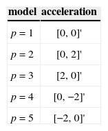
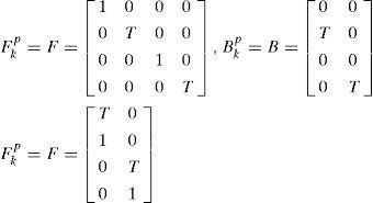
Where {x, y} are the Cartesian coordinates of target position in a 2D plane and {x˙,y˙} are the corresponding velocities. The target dynamic models are given in Equation 1 with five constant acceleration input levels u^p, which are given in Table 2. The matrices in Equation 1 are given below:

Table 2.

Acceleration input u^p

model	acceleration
p = 1	[0, 0]'
p = 2	[0, 2]'
p = 3	[2, 0]'
p = 4	[0, −2]'
p = 5	[−2, 0]'

Where T = 1s is the sample interval. Assume a linear measurement model (Equation 2):

The covariances of the process noise and the measurement noise are:

Note that the target follows an (almost) constant velocity (CV) model if the acceleration input is zero, and it follows an (almost) constant acceleration (CA) model for non-zero input. In each MC run, 45 steps are simulated. The target starts with the CV model and has random model switches at k = 16 and k = 30. The numbers of false measurements are i.i.d. Poisson distributed with spatial density λ. The false measurements are uniformly distributed over the surveillance region. Validation gate may be used to reduce the number of false measurements in the algorithm. All the filters have the same initial estimate

The true initial state of the target in each MC run is generated by:

Note that the set of target dynamic models used in each filter matches the model set of true target motion, that is, there is no model-set mismatch between the truth and filters. Admittedly, this is ideal and most often not true in practice. However, tackling the problem of model-set mismatch is beyond this work.

6.2

Performance measure

The following performance measures are evaluated:

• 1.

  Root mean square errors (RMSE) of position and velocity. They reveal the estimation accuracy of each algorithm.

• 2.

  Non-credibility index (NCI):

  

• 3.

  Inclination index (I.I.):

  

  Where

  

And [i] is the index of MC runs. The filter is credible if NCI is close to zero, meaning that the estimated MSE is close to the true MSE. I.I. shows the inclination (pessimistic or optimistic) of the filter. If I.I. is larger than zero, then the filter tends to be optimistic, meaning that the estimated MSE is smaller than the truth. If I.I. is smaller than zero, then the filter is pessimistic. See [34,35] for more details about NCI and I.I.

6.3

Comparative methods

Our method is compared with the following algorithms:

IMM+PDA: The IMM method is used to deal with the model uncertainty. The standard KF in IMM is replaced by the PDA filter which deals with the measurement origin uncertainty.

IMM+MHT: The MHT is modified by replacing KF by IMM. The numbers of hypotheses are reduced by GMR. Each Gaussian component corresponds to a hypothesis and is approximated by the fusion output of IMM.

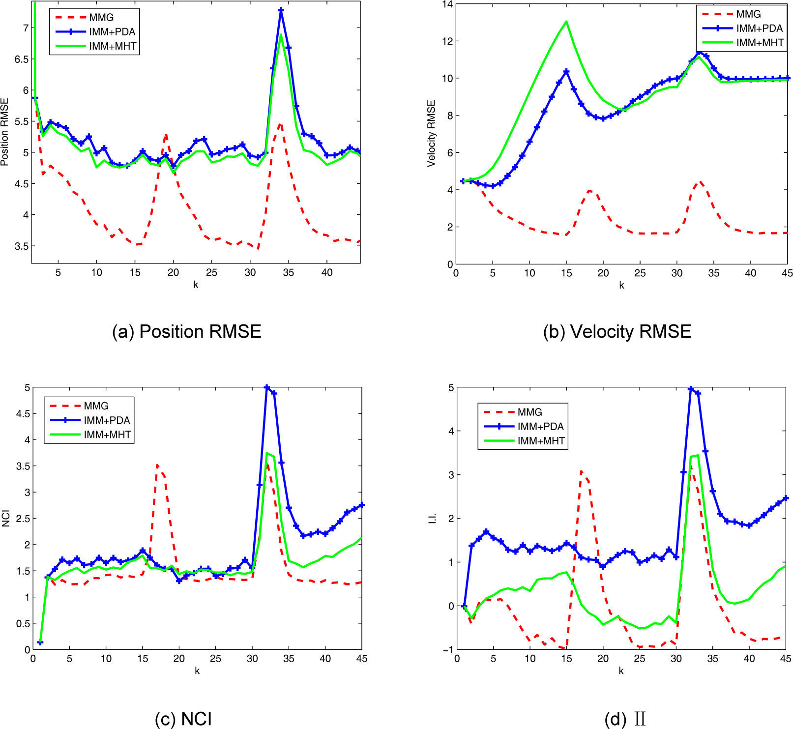
6.4

Simulation results

Case 1: A moderate density of clutter is considered. We set λ = 3 × 10⁻³ (unit m⁻²). M = 10 Gaussian components (or hypotheses) are maintained in MMG and IMM+MHT. The results are given in Figure 1. MMG has the best performance in terms of the position RMSE and velocity RMSE, where the two peaks of MMG correspond to the occurrences of model switch. The IMM based methods are more robust to the switch from CV model to the other models because there is no error peak at the time of the first model switch. Also, MMG has the lowest NCI for most of the time.

Figure 1.

Simulation results for Case 1. Figures. 1(a) and 1(b) show the position RMSE and velocity RMSE, respectively. The NCI and I.I. are given in Figures. 1(c) and 1(d), respectively. MMG has better performance for most of the time, except for the steps right after a model switch.

From I.I., it is clear that MMG is constantly pessimistic except at the transient steps while IMM+PDA is constantly optimistic. The IMM+MHT method does not show any consistent pattern.

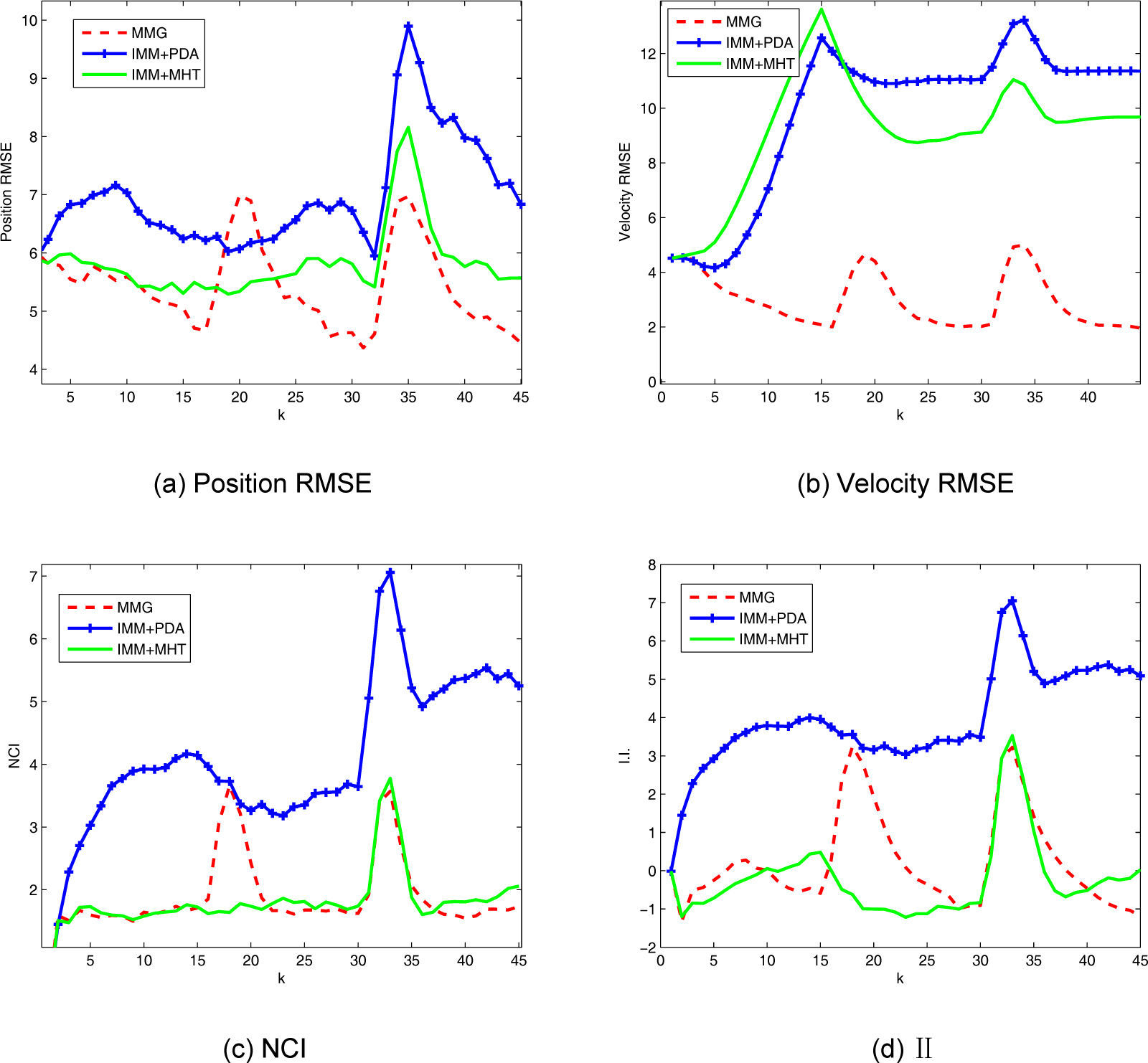
Case 2: The clutter density is increased to λ = 3 × 10⁻³ (unit m⁻² ). M = 15 components (or hypotheses) are maintained in MMG and IMM+MHT methods. Again, MMG outperforms the other two algorithms in terms of estimation accuracy for most of the time. Similar to Case 1, IMM+PDA and IMM+MHT are not sensitive to the switch from CV model to the other models. All the filters have larger estimation errors than those in Case 1. This makes sense due to the increase of clutter density. The NCI and I.I. of IMM+PDA become much worse than the other two algorithms, meaning that the PDA is more sensitive to the clutter density.

7

Conclusions

An algorithm (i.e., MMG) combining multiple model (MM) method and multiple hypothesis tracker (MHT) based on Gaussian mixture reduction (GMR) is proposed in this work to address the problem of single maneuvering target tracking in clutter. MM and MHT are two well-known methods to cope with the target model uncertainty and measurement origin uncertainty, respectively. Existing methods combined these two algorithms heuristically, where the number of hypotheses in MHT and the number of model trajectories in MM are reduced separately. In MMG, they are reduced jointly based on GMR. It is theoretically more appealing and has superior performance, which is demonstrated when comparing with the existing IMM+PDA algorithm and IMM+MHT algorithm.

Acknowledgments

This research was supported by the Fundamental Research Funds for the Central Universities (China), project No. 12QN41.