Education-earnings linkage for assessing societal benefits of interventions for children and youth in Sweden

Abstract

Some long-term societal benefits of early psychosocial interventions supporting children and youth at various developmental risks can be estimated with school results as a mediatory. In this paper we develop causal education-earnings links for educational achievement thresholds at the end of the nine-year compulsory school (CS) and the three-year upper secondary school (USS) in Sweden. Gross earnings are calculated with age profiles estimated on micro-level register data for the whole population. We also estimate the indirect costs of education (forgone earnings) with this data and find that they can be ignored. For the base case, we calculate the expected net present value of meeting minimum requirements for transition from CS to a national USS-program to €112,000 (SEK 1.1 million) and for graduation from such a program to €163,000 (SEK 1.6 million).

Resumen

Pueden calcularse algunos de los beneficios sociales a largo plazo de las intervenciones psicosociales precoces que respaldan a los niños y jóvenes con ciertos riesgos evolutivos utilizando los resultados escolares como hilo mediador. En este documento desarrollamos vínculos causales educación-ingresos para los umbrales del logro educativo al finalizar la escuela obligatoria (EO) de nueve años de duración y la escuela secundaria superior (ESS) en Suecia. Se calculan los ingresos brutos con los perfiles de edad estimados en un registro de datos a micronivel para la totalidad de la población. También calculamos los costes educativos indirectos (ingresos no percibidos) con estos datos, y encontramos que pueden ser ignorados. Para el caso básico, calculamos el valor actual neto previsto del logro de los requisitos mínimos para la transición de la EO al programa nacional de ESS de 112,000 € (1.1 millones de coronas suecas) y para la graduación en dicho programa de 163,000 € (1.6 millones de coronas suecas).

Introduction

Impact evaluations of psychosocial intervention programs for youth at developmental risks (for instance victims of school bullying, youth with mental health issues or foster children) are usually based on immediate or short-term follow ups, leaving it an open question whether the programs provide long-term societal benefits that make the programs worth spending of limited public budget money. To estimate such societal values it is necessary to predict long-term effects. This can be done, to some extent, by using the causal link between education and life-course earnings as a mediatory. In this study we develop such a linkage with data for the whole Swedish population.

The leading benefit-cost model for analysis of public policies targeting individuals at risk is a model that has been developed and is continuously updated by the Washington State Institute of Public Policy (WSIPP, 2016) for producing internally consistent estimates of benefits and costs of public policies for the Washington State legislature. Models in other US states and in the UK are to a large extent adaptations of this model (Little & Edovald, 2012; Pew, 2013), but these approaches have not so far spread out of the Anglo-Saxon world. The US models include an education-earnings link based on analysis of cross sectional annual data for earnings by age and educational status as reported in the US Census Bureau's March Supplement to the Current Population Survey (CPS). Similar calculations are made also for several European countries on an annual basis by the OECD in the yearbook “Education at a glance” (OECD, 2016). The WSIPP and OECD approaches have similarities and differences both in estimation of effects from education on life-course earnings and in calculation of the costs of education that to some extent reflect limitations of the source data. For instance WSIPP accounts for age but not gender, while OECD has it the other way around. OECD accounts for the opportunity cost of education from forgone earnings, while WSIPP ignores this item. Having access to register data for the whole Swedish population we are here able to overcome some of these limitations, not just with respect to inclusion of both age and gender. In particular, we find that in the Swedish context, the OECD approach to estimating the indirect costs of further education from forgone earnings exaggerates the opportunity cost component for secondary education.

In this study we develop links from two educational achievements to the net present value (NPV) of life-course gross income from earnings using micro-level data for the whole population in Sweden 2013. These achievements are (1) being eligible at the end of the nine years compulsory school (CS) to a national program in the three years upper-secondary school (USS), i.e., fulfilling some criteria based on the final credits from CS, and (2) graduation in USS. The first of these achievements is an educational milestone which can be observed with data from national registers in Sweden.

We calculate NPV from the incremental expected present value of gross earnings, net of public and private (opportunity) cost of education, from USS graduation. Following the WSIPP approach, incremental gross earnings are calculated from estimated age profiles based on micro-level register data for the whole Swedish population. This data also allows us to estimate the opportunity cost of education due to forgone earnings. A causality vs. correlation correction factor, based on Swedish studies, is used to account for selection effects. Further, we use cross-table statistics to compute the probabilities of graduation from USS and the expected time of USS education contingent on whether the eligibility threshold is passed or not.

Background

Introduction

The idea that wages includes an education premium was first suggested by Smith (1776/1974, pp. 203–204). The long pursuit for empirical estimates of the returns to education has been summarized in several papers (see for example Psacharopoulos & Patrinos, 2004). In general it is found that the rate of return to education is lower in more developed countries, lower for higher level of education and higher for women. On average the overall private rate of return to education is about 10 percent per year (Psacharopoulos & Patrinos, 2004). However the return to education differs depending on when it appears, and there seems to exist several “thresholds”, such as completion of a certain degree, that offer a larger return then just passing an extra year (Heckman, Lochner, & Todd, 2008).

Furthermore, a correlation between education and subsequent outcomes can be the result of selection and does not imply causality. Several studies have therefore used quasi-experimental approaches, such as natural experiments and matching based on twin registers (e.g., Aakvik et al., 2010; Isacsson, 1999; Meghir & Palme, 2005) to estimate the causal effects of education.

In benefit-cost analysis, effects of interventions are assessed according to how they contribute to aggregated societal welfare. This means that all real benefits and costs are included irrespective of whether they are private or public. The focus of this study is on possible effects on productivity over the life course of individuals who have received support from programs for children and youth at developmental risks that may harm their school achievements. If a causal education-earnings link can be established such productivity effects can be predicted from program impact evaluations that directly or indirectly can be related to school results. To construct such a linkage it is necessary to estimate the education premium for gross earnings (i.e., total wage cost to employers and earnings from self-employment, as a measure of productivity), the portion of this premium that is causal, and direct and indirect education costs. This can then be used to calculate the expected net present value of future earnings, conditional on the educational achievement. Two well-established ways to do this, fully or partly, are approaches used by OECD and WSIPP, respectively. They will now be described.

The OECD and WSIPP approaches

Each year OECD estimates the private and public financial returns from investments in education for its member countries (OECD, 2016). The private benefit is defined as the difference in expected net present value of life time earnings of individuals with different levels of education (primary, secondary and tertiary levels). In calculating this value OECD accounts for differences in income tax, transfers (unemployment benefits), social contributions and the probability to get a job. The public benefit is defined as the change of the NPV of tax revenues and social transfers.

On the cost side both the direct and indirect cost of education is considered. The private cost of education includes direct education-related household expenditure and indirect costs; i.e., the opportunity cost of time from forgone earnings of time spent in school instead of in work. The latter component is calculated by OECD as the minimum wage for a full-time job, net of income tax, times the probability to get a job. It is further assumed that students do not have any income while in school. For the government the cost of education is the money per student spent on education and the forgone tax income while the student is in school. By adding the public and private return the social return to education can be held. The annual statistics provided by the OECD is presented separately for men and women. It can further be noticed that the OECD does not use a causality correction factor, does not account for mortality, and uses a 2 percent rate of discount.

The benefit-cost model used by WSIPP (2016) includes an education-earnings module that estimates the increase of life-course labor market earnings as a consequence of having a high school graduation or another year of education. The effect on earnings is calculated from analysis of cross sectional data (US Census population survey) for individuals aged 18–65 (including people with zero earning). While the approach is cross-sectional, data from several years, separated by year-dummy variables, is used so as to capture a whole business cycle. The most recent estimate is based on data from 2002 to 2010. With this data, age-earning profiles, contingent on educational status, are estimated by OLS regression.

Since the census does not include employee benefits (paid leave, supplemental pay, insurance, retirement and savings, and legally retired benefits) a correction for such earnings is made by estimating the ratio of employee compensation from the data “Employer costs for Employee Compensation” to wage and salaries (1.441). This is then added to the earnings from the census data.

The age profiles are used to calculate gross benefits of educations as the expected present value of earnings (2003–2010) for varying rates of discount (2%, 3.5%, 5%) and assumptions about the future annual real growth rate of earnings (0.53%). Future earnings are contingent on survival, so expected values of these earnings are computed using mortality rates at different ages (years).

The difference in earnings over the labor-market active life span between age-profiles for different levels of education is then used to calculate the present value of incremental earnings from an additional level of education. However, having a high school graduation also gives access to higher level of education. Therefore it would be misleading to compare the ones with USS as their highest level of education with the ones with no secondary education to value the benefit from USS. To capture this the model includes an estimate of the share of students passing to the next level of education and the change of life time earnings that such progress induces.

WSIPP corrects the education gross benefit for causality by a causality factor derived by Heckman et al. (2015). Finally, WSIPP calculates the net benefit from an increase in education from the causality-adjusted gross benefit by subtracting the average public direct cost of education per student, with separate estimates for low income students and special education. Thus, in contrast to the OECD, private expenditure is not included and no account is taken of private or public forgone earnings.

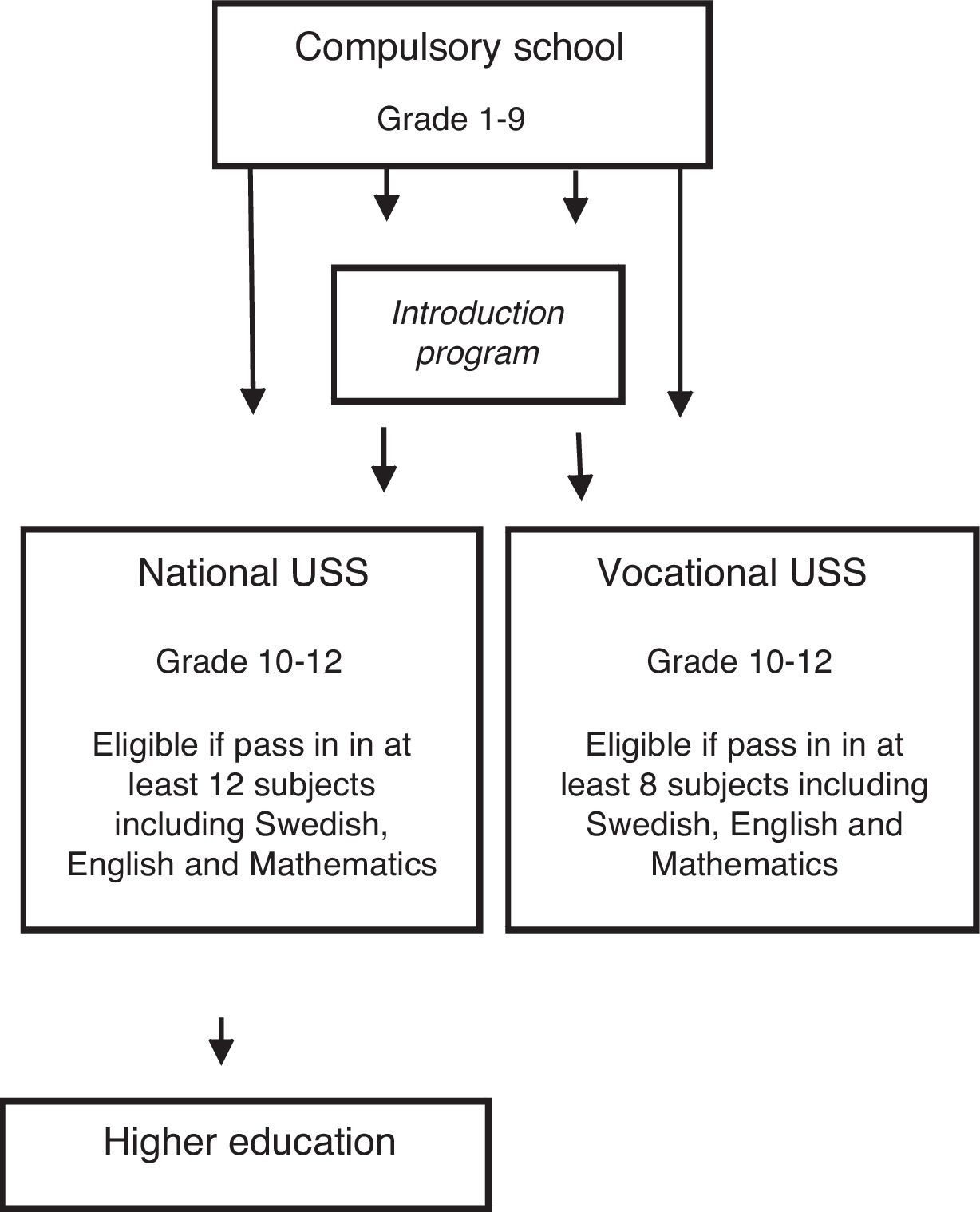
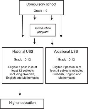
The Swedish context

On the Swedish labor market an exam from USS is required for many jobs, even for those that do not require specific vocational or academic education (Arbetsförmedlingen, 2016), so being eligible to at least a vocational USS program is a major threshold achievement in the CS and then at the next level of course to actually graduate from USS. The three years national USS programs in Sweden are voluntary. USS education is offered in Sweden free of charge by both private (companies or non-profit institutes) and public schools. As shown in Fig. 1, the student can choose to enter either a vocational USS, which prepares the student for the labor market, or a national USS, which gives the student access to higher education. To be eligible to a vocational USS national program a pupil must finish grade 9 (normally at age 15–16) with a pass in at least 8 subjects including Swedish (or Swedish as a Second Language), English and Mathematics. To be eligible to a national USS, a pass is needed in at least 12 subjects (a student normally gets 16–18 grades). After they finish CS 99.5 percent of all pupils¹ continue within two years from grade 9 to the USS (Government Report 2016). However, only about 85 percent of these pupils are eligible to a direct start. The non-eligible pupils start instead in a so called Introduction program in which they are given a customized set of supplementary courses that is intended to give them possibility to later on transfer to a national or vocational program. Depending on the progress in the introduction program a few pupils catch up fast and finish USS within three years, while others begin in the national program after one or two years in the introduction program and can thus graduate USS after four or five years. However, the majority, drops out of the USS at some stage, sooner or later.

Fig. 1.

Overview of transition between primary, secondary (USS) and tertiary education in Sweden.

While close to all start in the USS, just about two thirds graduate after three years. Table 1 shows statistical records from 2012. Of those who started three years earlier (2009) 68 percent graduated this year, while of those who had started three to five years earlier (2007–2009), 77.5 percent graduated in 2012. However, there was a marked difference between those who were admitted from the start to a national program and those who were not. Among the latter only 5.5 percent and 26 percent graduated within three and five years, respectively. Female graduation rates are in general about ten percent higher than those of males, but there is no clear gender difference in these proportions among those who follow the vocational programs.

Table 1.

Average probabilities of completing USS in 3 or 4–5 years conditional on being eligible to a national USS program. Percent.

Status at end of CS	USS 3 years	USS 4–5 years	No USS exam
Eligible to national program	68	11.5	22.5
Non-eligible	5.5	20.5	76

Source: Gymnasieutredningen (2016).

Of those who never graduate some leave school early. Of those who started in a national program in 2013, 2 percent dropped out during the first two years. The corresponding proportion of early school leavers among pupils starting in the Introduction program (i.e., those who were not eligible to a national program) was 24 percent (Gymnasieutredningen, 2016, p. 183).

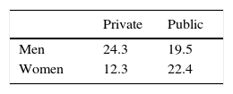
Implications for estimation of the societal benefits of education in Sweden

Table 2 shows a recent estimate by the OECD of the private and public rates of return to upper secondary education in Sweden for male and female students. These returns are estimated as net present value differences of revenues and costs compared to when the student finishes directly after the CS (primary level).

Table 2.

Rate of return to upper secondary education (but no tertiary education) in Sweden percent.

	Private	Public
Men	24.3	19.5
Women	12.3	22.4

Source: OECD (2016).

It can be noticed that the private return (private) to USS for women in Sweden is only 61 percent of the respective number for men, while the public rate of return is instead found to be larger for women than for men.

However, from the description of the Swedish context in the previous section it is clear that the real difference in the direct costs of education between those who graduate from the USS and those who do not is smaller than the OECD estimates, since close to all students spend at least some time in USS education even if they do not graduate. Moreover, according to OECD the indirect cost of education (forgone earnings) amount to about 80 percent of the direct cost. This can be questioned since OECD ignores earnings by students during vacations and other spare time.

Also, in the Swedish context, a main delineation seems to be between those pupils that leave the ninth year of CS being eligible to a national program and those who are not eligible. For programs supporting children in early years at some developmental risk, this eligibility is an important outcome variable that affects societal benefits and costs on the long term. Estimating benefits and costs conditional on such eligibility is therefore the main focus of our empirical study.

A major methodological challenge is the treatment of the option value of education, i.e., the value of the possibility to continue to education at a higher level. For instance, some USS drop-outs will probably return to school some years later to get a USS degree and in that case the age profile wage differences between CS and USS individuals overestimates the life-courses earnings difference. On the other hand, a portion of those with USS education will later continue to tertiary education, implying underestimation of life-course earnings. In a societal benefit-cost perspective even more complexity is added by the need to also consider the direct and indirect public and private costs of the subsequent education for both groups. The OECD does not include these option values but calculates separately education premia for tertiary education, while WSIPP includes the benefit part of the option value from high school education (but not for primary education).

In this study, we have chosen to ignore these option values. We will compare annual earnings of individuals with CS or USS as their highest educational attainments. This is equivalent to assuming that, in a societal perspective, the option value (net present value from subsequent education) for those with a USS degree but (not yet) more is equal to the value (net present value from subsequent education) of those with a CS education but (not yet) a USS degree. Besides simplicity, there are two main arguments for this approach. First, since the number of people continuing to tertiary education after USS is larger than of those who complete USS as adults, and because those who reach the highest wage levels tend to be in the first category, we avoid exaggerating benefits. Second, this approach is more relevant for evaluation of benefits from interventions that help children and youth to reach just over the eligibility threshold.

We therefore first estimate the incremental earnings in a comparison of individuals for which the highest educational attainment is either CS or USS. We use Swedish data that allows for consideration of both age profiles and gender differences. With this data we also investigate what the actual differences are in earnings during the ages 16–19 of those have graduated from USS at age 20 and those who have not. Finally, we calculate expected NPV of passing the eligibility threshold, based on the average success frequencies in USS that were reported in the previous section.

Earnings age profiles

This section describes the statistical models, the data and the results from estimation of age profiles for the Swedish population in 2013 depending on educational status.

Method

To estimate the earnings age profiles we divide the sample into groups based on their age and level of education. The first age group consist of individuals aged 20–65, which means that they most likely are in the labor force or in higher education. The other age group consists of individuals aged 16–20, which means that they most likely have finished the CS, but might still be in USS. These two groups are then further divided according to their level of education where individuals in the first group only have CS education and the others have USS education (but no higher education). We start by estimating the life-course earnings age profiles for individuals aged 20–65:

where E_iy is the gross annual earnings for individual i in year y. To control for the influence of the business cycle we use data for year 2010–2013 and include year dummies for each year (the reference year is 2013). Group A consists of individuals with USS education and group B consist of individuals with only CS education.

To estimate the earnings of individuals who might still be in USS (age 16–20) we start by identifying individuals who are 20 or 19 years old in year 2013, respectively, and whose occupation was not recorded as student in November that year. We then divide them into individuals who have at least some USS education (but no higher education) (group C) and individuals who only have CS education (group D). We then estimate their earnings age profile for the previous four, respectively three, years (i.e., for when they were 16–19, respectively 16–18, years old which is the age when we expect them to be in USS):

In this way we can find the earnings for young people who after CS do not continue to USS during the years when their peers still are in USS and for youth who still are in USS. The difference in earnings for these two groups is the opportunity cost of USS.

To control for difference in earnings between male and female students we run all the regressions split on gender.

By combining the result for the different groups we can estimate the age-earning profiles for individuals with only compulsory education and for those with USS education (but no higher education). This can then be used as a base to estimate the expected change in life time earnings from an increase in education.

Data

The earnings, age and education data is compiled from LISA, a longitudinal database administered by Statistics Sweden (SCB 2016). LISA contains information on all individuals 16 years of age and older that were registered as resident in Sweden as of December 31 for each year.

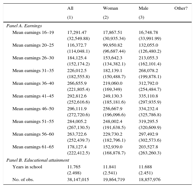
The earnings variable is the sum of labor income and earnings from self-employment. Labor income refers to total gross annual labor income from all sources. Education is reported in accordance with the SUN2000 (Svensk utbildningsnomenklatur), which corresponds to the International Standard Classification of Education 1997 (ISCED-97) (Halldén, 2008). For each individual and year SUN reports the highest completed education according to a 3-digit classification. The first digit gives the level of education, the second the number of years in school, the third the type of education. For example the SUN2000 code 337 corresponds to upper secondary school, three years, vocational education (“gymnasial treårig yrkesinriktad utbildning”). A descriptive summary of the data used in the estimation of age earnings profiles is displayed in Table 3.

Table 3.

Descriptive statistics, earnings by age and sex, 2009–2013. Averages (standard deviations in parentheses). SEK/year.

	All	Woman	Male	Other?
	(1)	(2)	(3)
Panel A. Earnings
Mean earnings 16–19	17,291.47 (32,549.88)	17,867.51 (30,935.34)	16,748.78 (33,991.99)
Mean earnings 20–25	116,372.7 (114,048.1)	99,950.82 (96,687.44)	132,055.0 (126,480.2)
Mean earnings 26–30	184,125.4 (152,174.2)	153,642.3 (134,382.1)	213,055.3 (162,101.4)
Mean earnings 31–35	226,012.5 (182,555.8)	182,139.1 (150,488.7)	268,078.2 (199,878.1)
Mean earnings 36–40	266,655.9 (221,805.4)	219,060.0 (169,349)	312,792.0 (254,484.7)
Mean earnings 41–45	292,812.6 (252,616.6)	249,130.3 (185,181.6)	335,110.8 (297,935.9)
Mean earnings 46–50	296,111.9 (272,720.6)	256,667.9 (196,096.6)	334,232.4 (325,786.8)
Mean earnings 51–55	284,005.2 (267,130.5)	248,002.4 (191,638.5)	319,295.5 (320,609.9)
Mean earnings 56–60	263,722.6 (252,439.7)	229,730.2 (182,796.1)	297,492.9 (302,573.6)
Mean earnings 61–65	178,127.4 (222,412.5)	152,939.0 (168,878.7)	203,527.8 (263,260.3)
Panel B. Educational attainment
Years in school	11.765 (2.498)	11.841 (2.541)	11.688 (2.451)
No. of obs.	38,147,015	19,864,719	18,857,976

Note: Earnings are total income from employment and self-employment, based on tax reports. Source: The Swedish Tax Agency (Skatteverket).

Age earnings profiles results

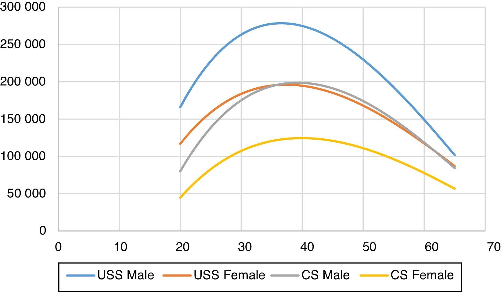
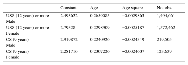
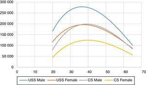
The age earnings profile estimates are shown in Table 4 and depicted in Fig. 2. It can be seen that there are marked differences in annual earnings between gender and between with CS or USS education. In fact, the gender gap is more or less equal to the education gap. All age profiles have a marked concavity. The CS wages peak at around 47 and the USS at around 45.

Table 4.

Estimated age profiles for the whole Swedish population 2013, 20–65 years old. 100 SEK/year.

	Constant	Age	Age square	No. obs.
USS (12 years) or more Male	2.493622	0.2659085	−0.0029863	1,494,661
USS (12 years) or more Female	2.79328	0.2298909	−0.0025187	1,572,462
CS (9 years) Male	2.919872	0.2240926	−0.0024349	219,505
CS (9 years) Female	2.281716	0.2307226	−0.0024607	123,639

Fig. 2.

Age profiles for annual earnings 2013 for the total Swedish population conditional on highest educational status the same year (CS = compulsory school; USS = upper secondary school).

Forgone earnings

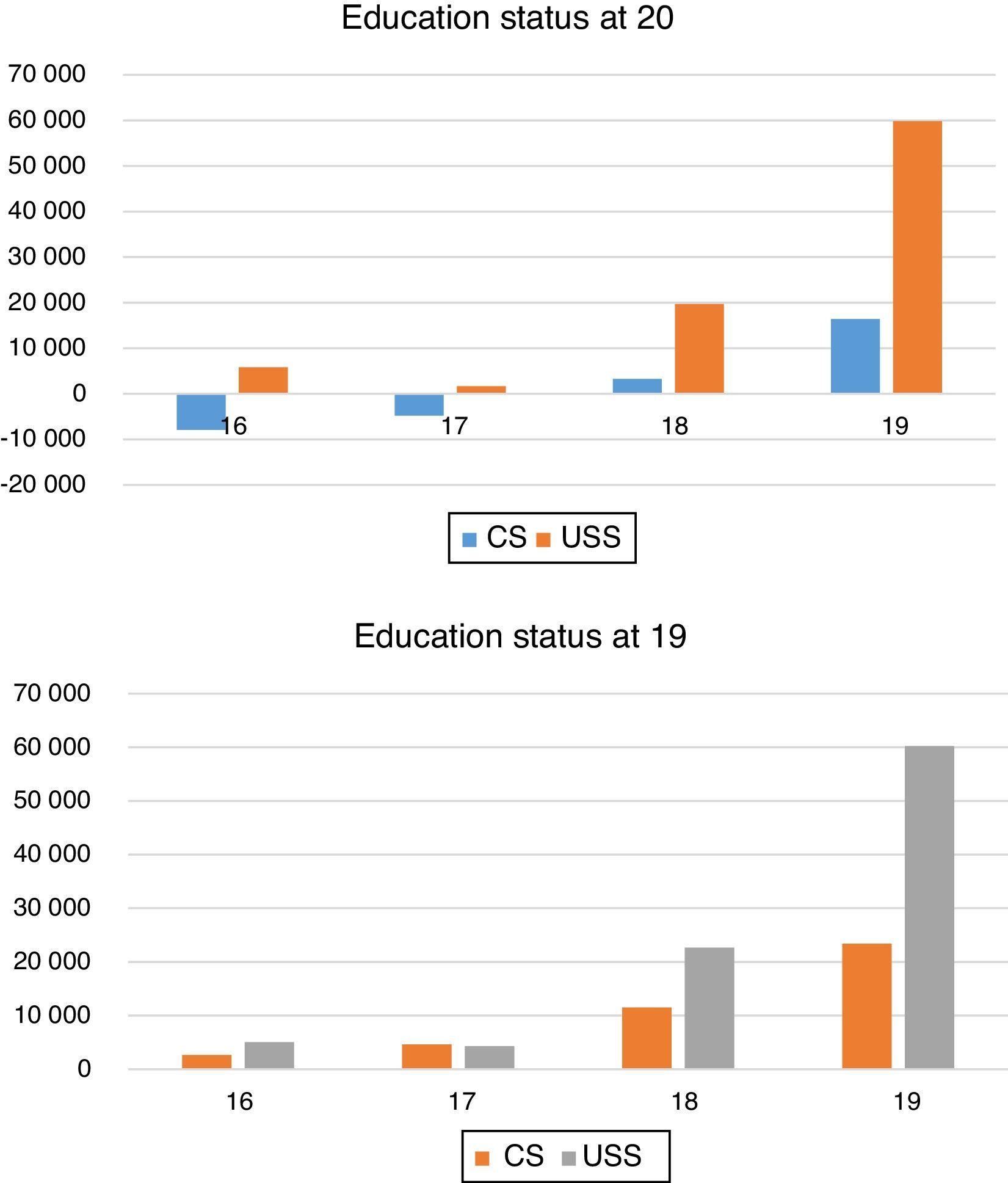
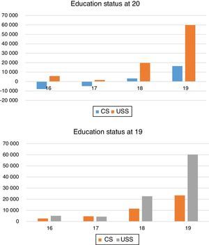
Forgone earnings are the earnings that a student forgoes by spending time at school instead of working. To estimate these for USS students, we have calculated the annual earnings at age 16, 17, 18, 19 and 20 of those in the Swedish population in 2013 that were 20 or 19 years old, so that the average earnings at these ages can be compared between those who at 20 had completed the USS to those who at that age had not completed the USS. Since the majority of USS students finish the year they reach age 19, the differences in earnings at age 16, 17, 18 and possibly 19 could be expected to reflect the forgone earnings cost of education. Even if USS students are able to do some work, especially during the summer holidays, obviously a USS drop-out student has more time that could be used for working.

The results are shown in Fig. 3. As can be seen, contrary to the perhaps naïve expectation, people that at age 20 had graduated from USS had received higher earnings during the USS ages than the non-graduates. Similar results are held for those who were 19 years old (notice that the negative values for the 19 years old at ages 16 and 17 are an artifact of fitting a second-degree polynomial to the data). As was mentioned above, close to all individuals continue from CS to USS. Clearly from Fig. 2 those who drop out do not on average get more earnings from work than those who stay and finish USS. On the contrary they get less, which suggests a disadvantage in “employability” even for temporary work during school vacations, etc. For the purpose of cost-benefit analysis it can be concluded that in the current Swedish context no large error will be made by simply ignoring the forgone earnings cost of USS education.

Fig. 3.

Annual earnings (SEK) at ages 16–19 of individuals that 2013 were of age 20 or 19, respectively, with different educational status (not being registered as students in November 2013 and with USS or CS as highest educational status).

Net present value of educational achievements

This section describes the calculation of the NPV of, first, USS graduation and, second, of eligibility to a national USS program. All present values are expected averages contingent on educational achievement, evaluated at the age of 16 (i.e., when an individual finishes CS).

NPV models

The gross societal present value of an expected education differential (i.e., the education premium including both public and private benefits) at age 16 is calculated by first taking the difference in average earnings between groups of individuals with different educational status at all ages between 20 and 65, multiply by the conditional probability of survival until a specific age in this interval, discount to age 16, and finally multiplying by the payroll tax factor to get the present value of gross earning. Thus we compute first

and then

where π[age] is the probability at age 16 of survival until a specific age, r = δ − g is the effective rate of discount, the difference between the social discount rate δ and the expected constant exponential real rate of growth of wages g and τ is the payroll tax. The payroll tax in Sweden is 30.52%.

The incremental NPV of USS graduation (12 years) when the alternative is CS (9 years) is derived by subtracting the present value of the education costs, i.e.,

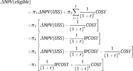
where ω is the causality/correlation correction factor, COST is the average annual cost of a USS program. ΔPV(CS) is the present value of forgone earnings, which will not be described further as it will be hereafter ignored, based on the empirical finding reported above. This implies that while the first term includes both private and public benefits, all costs are represented by the second term.

The next step is to calculate the expected incremental NPV of being eligible to at least a vocational national USS program. Based on the frequencies shown in Table 1, this is computed as

where IPCOST is the average cost of the Introduction program and T > 3 is the average number of years for graduation from USS for those who do not graduate after three years and π₁ to π₅ are the probabilities shown in Table 1.

Causality

Based on a summary of previous Swedish literature Björklund, Fredriksson, Gustafsson, and Öckert (2010) concludes that the casual part of the relationship between education and earnings is around 0.5. This is consistent with the value used by WSIPP (Mean 0.5, SE 0.17) based on the analysis by Heckman et al. (2015).

This portion is somewhat corroborated by a recent study based on Swedish data (Lång & Nystedt, 2016). Using data for the whole Swedish population 18–75 years old, it is estimated that an additional year of schooling for males is associated with around 5–6 percent higher earnings from age 35 onward and with 6 percent higher earning for females. These analysts then do similar estimations for a large set of dizygotic (DZ) and monozygotic (MZ) twins, which makes it possible to make within twin pair comparisons and thereby control for differences in family conditions (DZ and MZ) and genetic conditions (MZ). They find that the estimates for the DZ twin pair sample are lower by on average 25 percent for ages 30–75, while the corresponding reduction for the male MZ twin pairs is 65 percent and 50 percent for females (the differences between estimates for the DZ and MZ twin samples are statistically significant only for males).

In this study or base calculations we use a causality correction factor of 0.5, but in a sensitivity analysis we also use 0.35 (corresponding to a 65 percent reduction). We do not consider side effects or external benefits.

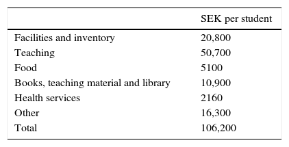
Education costs

The private cost of USS education will here be assumed to be zero. There are no tuition fees and as concluded above the forgone earnings can be ignored. The remaining cost is the public cost, which is borne by the municipality. This cost was on average 106200 SEK (Skolverket, 2017a). This average cost includes fixed and joint cost components and is therefore not necessarily equal to the marginal cost. A decomposition in various cost items is shown in Table 5. However, for the purpose of the present study we use the total average cost.

Table 5.

Annual costs per USS student. National average 2013, SEK/student.

	SEK per student
Facilities and inventory	20,800
Teaching	50,700
Food	5100
Books, teaching material and library	10,900
Health services	2160
Other	16,300
Total	106,200

Source: Skolverket (2017a).

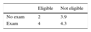
For all USS students that were not initially eligible to a national program the education cost is increased by 40,000 SEK, which is assumed to be the cost of additional education to fill the requirements for continuing in a national program. Further, we make assumptions regarding the average number of years in USS as shown in Table 6:

Table 6.

Assumed number of years in USS of various categories of pupils.

	Eligible	Not eligible
No exam	2	3.9
Exam	4	4.3

Source: Own calculations based on Skolverket (2017b).

Results

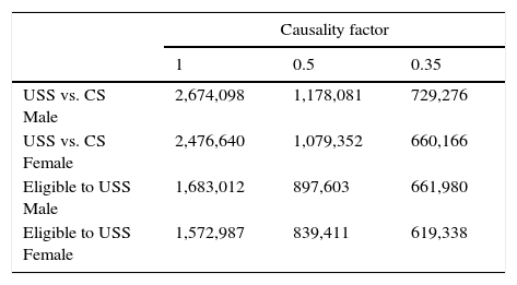
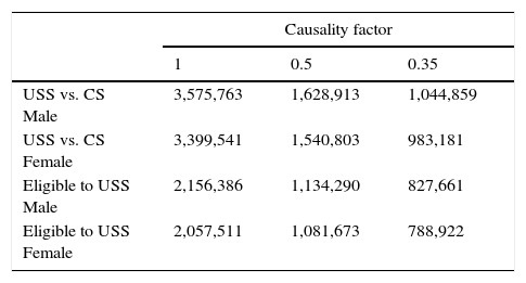
Based on the results from the estimated age-earnings profiles (Table 4) and the average transition probabilities shown in Table 1, we have calculated the expected net present values for male and females, respectively, shown in Tables 7a and 7b. Table 7a reports results using a standard discount rate of 3 percent and zero average real wage growth. The Swedish National Transport Administration (Trafikverket, 2016) assumes 1.5 percent real wage growth in benefit-cost evaluations of infrastructure projects for the period 2014–2060. Table 7b therefore shows results for 1.5 percent expected real wage growth, thus with an effective discount rate of 1.5 percent. Earnings at all ages are adjusted by average survival probabilities of the Swedish population, conditional on being 16 years age old (Statistics Sweden, 2017). Results are reported for three causality correction factors 1, 0.5 and 0.35.

Table 7a.

Incremental societal net present value of passing an educational threshold: USS graduation and eligibility to national USS program. Swedish kronor (SEK) at 3 percent rate of discount, evaluated at age 16. Real wage growth 0%.

	Causality factor
	1	0.5	0.35
USS vs. CS Male	2,674,098	1,178,081	729,276
USS vs. CS Female	2,476,640	1,079,352	660,166
Eligible to USS Male	1,683,012	897,603	661,980
Eligible to USS Female	1,572,987	839,411	619,338

Table 7b.

Incremental societal net present value of passing an educational threshold: USS graduation and eligibility to national USS program. Swedish kronor (SEK) at 3 percent rate of discount, evaluated at age 16. Real wage growth 1.5%.

	Causality factor
	1	0.5	0.35
USS vs. CS Male	3,575,763	1,628,913	1,044,859
USS vs. CS Female	3,399,541	1,540,803	983,181
Eligible to USS Male	2,156,386	1,134,290	827,661
Eligible to USS Female	2,057,511	1,081,673	788,922

Taking the results with a 0.5 causality correction factor and 1.5 percent real wage growth as the base case, we find that the expected net present societal value of completing a USS education (evaluated at age 16) is around 1.6 million SEK (Euro 163,000) and the expected net present societal value of being eligible to a national USS program is around 1.1 million SEK (Euro 112,000). The gender differences are small, indicating that that the gender wage gaps are of similar magnitudes for earners with USS education compared to those with only CS education. These average values for both genders are reduced to 1 and 0.8 million SEK (Euro 102,000 and 82,000) for a lower causality correction factor (0.35) and to 1.1 and 0.86 million SEK (Euro 112,000 and 88,000) for zero wage growth.

Discussion

In this study we are interested in the education-earnings link as a means for conducting societal benefit-cost analysis of prevention and early intervention measures for children and youth at various kinds of risks and where the intervention impact can be linked to the probability of meeting the requirements for being eligible to a national USS program at the end of the CS. Our main finding is that the societal NPV of completing the USS is around 1.6 million SEK and of being eligible to a national USS program is close to 1.1 million SEK. Although there is a substantial wage gender gap, the gender differences in these net present values are small. These values are evaluated as expected net present values with a 3 percent rate of discount for individuals at the end of CS, i.e., at age 16, and with correction for expected mortality at various ages, expected real wage growth (1.5 percent) and a causality portion of the education premium at 50 percent. They can easily be changed with another set of parameters.

Some assumptions that have to be made in a calculation of this sort may seem quite innocent but have a substantial impact. An example is the procedure used by the OECD in calculation of education premia. The idea that forgone earnings are a considerable part of the cost of education has a long standing in economics (e.g., Mincer, 1958). However, this opportunity cost is difficult to estimate, and while it is ignored by WSIPP we think that the OECD approach has some weaknesses. We did not find evidence that there is a substantial such cost in the case of USS education in Sweden, which contrasts to the OECD results for Sweden, where this indirect cost of education amounts to 80 percent of the direct cost.

A related issue is how to account for subsequent education. We have chosen to estimate the earnings-age profiles from data for people with at most 12 years education, thereby excluding individuals that change to a higher educational level and, probably, on average get higher earnings. An alternative route is to add the net present value of subsequent education for a portion of those who have graduated at each education level. However that raises a range of difficult estimation issues, including assessment of the opportunity cost, accounting for differences in timing and time length of the subsequent education (many university students work part time, some study on their free time and work full time), etc. This opens many possibilities for making errors. An advantage of the approach taken here, besides simplicity, is that, the estimated net present values are likely to be on the low side. We expect the ignored option value of continuing to tertiary education after secondary education to be higher than the ignored option value of completing secondary education at a later point of time, since the benefit (education premium) is larger in the first case and while the direct cost of university education is on average lower than the direct cost of USS education.

Conclusions

The WSIPP approach for program evaluations has been implemented in a European context so far only in the UK (Little & Edovald, 2012). A core component of this approach is the causal link between children and youths’ achievements in school, which can be measurably impacted by early psycho-social interventions, and life-course earnings. In this study we have calculated how the expected societal NPV at age 16 from life course earnings is affected by whether or not a pupil meets the basic credit-rating requirements for being eligible to a national USS program. We have also calculated corresponding values for the USS education differential (compared to having only CS education). While several other studies have estimated USS differentials, they focus on the earnings (or wage) differentials and ignore expenditure cost. An exception is OECD (2016), which on the other hand, according to our findings, seems to exaggerate the relevant education cost. Also, for the purpose of economic evaluation of early psycho-social interventions, educational achievements at a younger age than after 12 years in school, such at age 16, can be more useful.

In this study we use cross-sectional evidence to predict future earnings differences. In a small open economy like Sweden the development over the long term of these differences depends on general trends of technological change on the global scale (Helpman, 2016). The dominant view on these trends seems to be that a previous tendency of skill-biased technical change, which increases education-related earnings differences, has been replaced by a task-biased technical change leading to job polarization, with expansion of the highest and lowest paid jobs compared to middle-wage jobs. Adermon and Gustavsson (2015) find evidence of such a development in Sweden during the 1990s and first five years of the current century. However, they also report that the growth of less qualified jobs seems to have been slow during the last 15 years. Bengtsson et al. (2014) using more recent data find small changes of wage differences but large changes of income differences during the 00s. While incomes of people with secondary and/or tertiary education have had a very favorable turn-out, incomes of both men and women with low education (i.e., lacking USS education) have been stagnant and were only slightly higher in 2012 compared to 1990. Therefore if this trend continues we can expect that the future earnings differences may become even larger than those that have been estimated here.

Clearly, the analysis made here can be extended in various directions. First, we have focused on effects of education on earnings, ignoring other possible social benefits, such as effects on health, criminality, etc. Nor do we have considered external benefits (Acemoglu & Angrist, 2000). However, in a recent review of the literature on such externalities, including some studies using Swedish data, Stenberg (2013, pp. 129–131) finds it inconclusive, and WSIPP introduces this aspect by sensitivity analysis only. Second, we have focused on two specific educational thresholds, i.e., eligibility to a national USS program and completion of USS education. For benefit-cost assessments of specific programs for children and youth even earlier achievements may be relevant, such as credit ratings at the sixth grade (which is the first grade in Sweden in which pupils get ratings), or results in specific cognitive and/or non-cognitive tests. Third, we have focused on averages, assuming that anyone who passes a specific education threshold has equal probabilities as anyone else passing this threshold. Clearly, this assumption could be questioned in several evaluation situations, for instance when the specific risk factor that is targeted by an intervention is correlated with general cognitive or non-cognitive individual characteristics that may influence the chances on the labor market.

However, building on the work reported here it should be possible to make elaborations to derive benefit-cost estimates that are perhaps better adapted to evaluation of specific programs. Also, benefit-cost evaluations always contain uncertain parameters and should therefore be regarded as a way to get the orders of magnitude right, not the very precise numbers. We believe that the estimates presented here can provide fruitful starting points in economic evaluation of psychosocial interventions if this is held in mind.

Conflict of interest

The authors have no conflict of interest to declare.